- Home
- About Journals
-
Information for Authors/ReviewersEditorial Policies
Publication Fee
Publication Cycle - Process Flowchart
Online Manuscript Submission and Tracking System
Publishing Ethics and Rectitude
Authorship
Author Benefits
Reviewer Guidelines
Guest Editor Guidelines
Peer Review Workflow
Quick Track Option
Copyediting Services
Bentham Open Membership
Bentham Open Advisory Board
Archiving Policies
Fabricating and Stating False Information
Post Publication Discussions and Corrections
Editorial Management
Advertise With Us
Funding Agencies
Rate List
Kudos
General FAQs
Special Fee Waivers and Discounts
- Contact
- Help
- About Us
- Search


Current Chemical Genomics and Translational Medicine
(Discontinued)
ISSN: 2213-9885 ― Volume 12, 2018
A Grid Algorithm for High Throughput Fitting of Dose-Response Curve Data
Yuhong Wang*, Ajit Jadhav, Noel Southal, Ruili Huang, Dac-Trung Nguyen
Abstract
We describe a novel algorithm, Grid algorithm, and the corresponding computer program for high throughput fitting of dose-response curves that are described by the four-parameter symmetric logistic dose-response model. The Grid algorithm searches through all points in a grid of four dimensions (parameters) and finds the optimum one that corresponds to the best fit. Using simulated dose-response curves, we examined the Grid program’s performance in reproducing the actual values that were used to generate the simulated data and compared it with the DRC package for the language and environment R and the XLfit add-in for Microsoft Excel. The Grid program was robust and consistently recovered the actual values for both complete and partial curves with or without noise. Both DRC and XLfit performed well on data without noise, but they were sensitive to and their performance degraded rapidly with increasing noise. The Grid program is automated and scalable to millions of dose-response curves, and it is able to process 100,000 dose-response curves from high throughput screening experiment per CPU hour. The Grid program has the potential of greatly increasing the productivity of large-scale dose-response data analysis and early drug discovery processes, and it is also applicable to many other curve fitting problems in chemical, biological, and medical sciences.
Article Information
Identifiers and Pagination:
Year: 2010Volume: 4
First Page: 57
Last Page: 66
Publisher Id: CCGTM-4-57
DOI: 10.2174/1875397301004010057
Article History:
Received Date: 13/7/2010Revision Received Date: 4/8/2010
Acceptance Date: 30/8/2010
Electronic publication date: 21/10/2010
Collection year: 2010
open-access license: This is an open access article licensed under the terms of the Creative Commons Attribution Non-Commercial License (http://creativecommons.org/licenses/by-nc/3.0/) which permits unrestricted, non-commercial use, distribution and reproduction in any medium, provided the work is properly cited.
* Address correspondence to this author at the National Institutes of Health, NIH Chemical Genomics Center, 9800 Medical Center Drive, Rockville, MD 20850, USA; Tel: 215-358-0186; Fax: 301-217-5728; E-mail: wangyuh@mail.nih.gov
| Open Peer Review Details | |||
|---|---|---|---|
| Manuscript submitted on 13-7-2010 |
Original Manuscript | A Grid Algorithm for High Throughput Fitting of Dose-Response Curve Data | |
1. INTRODUCTION
The technological advances in high throughput screening (HTS) [1Liu B, Li S, Hu J. Technological advances in high-throughput screening Am J Phamacogenomics 2004; 4: 263-76.] shifted the rate-limiting step in drug discovery from data generation to data analysis. In today's drug discovery process, thousands of dose-response curves are routinely generated in a typical secondary screening project. At the National Institutes of Health Chemical Genomics Center (NCGC), we have developed a new quantitative high-throughput screening (qHTS) paradigm [2Inglese J, Auld DS, Jadhav A, et al. Quantitative high-throughput screening: A titration-based approach that efficiently identifies biological activities in large chemical libraries Proc Natl Acad Sci USA 2006; 103: 11473-8.] to profile every compound in large collections of chemicals and search for chemical compounds of great potential in probing the chemical, genomic and biological universes and thus the biological pathways. In this new paradigm, compound titration is performed in the primary screening, and hundreds of thousands of dose-response curves are routinely generated.
High throughput curve fitting and outlier detection of such amount of dose-response data remain a great challenge [3Motulsky HJ. Fitting models to biological data using linear and nonlinear regression: a practical guide to curve fitting In: USA: Oxford University Press 2004.,4Motulsky HJ, Ransnas LA. Fitting curves to data using nonlinear regression: a practical and nonmathematical review FASEB J 1987; 1: 365-74.]. First, the current nonlinear curve fitting algorithms, such as Levenberg–Marquardt (LM) algorithm [5Levenberg K. A Method for the Solution of Certain Non-Linear Problems in Least Squares Q Appl Math 1994; 2: 164-8.], are based upon derivatives, their solutions correspond to local optimum, and the quality of the solutions to a large degree depends upon data quality and starting point. To find a good curve fit and solution, outlier data points, a common phenomenon for HTS data, need to be manually detected and masked, and different starting points need to be tried. As a consequence, these algorithms are difficult to automate and are generally not scalable.
A number of computer programs are currently available for fitting dose-response curves. The most widely used programs are the package DRC [6Ritz C, Streibig JC. Bioassay analysis using R J Stat Softw 2005; 12: 1-22.], an add-on for the language and environment R [7R Development Core Team. R: A language and environment for statistical com- puting. R Foundation for Statistical Computing, Vienna, Austria 2005 http://www.R-project.org ISBN 3-900051-07-0 ], and XLfit(R), a Microsoft(R) Excel add-in (www.idbs.com). The XLfit add-in is very popular in pharmaceutical and biotech industries, and the DRC package is used more in academic and government research institutions.
In this study, we proposed a novel algorithm, the Grid algorithm, for high throughput curve fitting. We will describe the algorithm and its performance first and then compare it with DRC and XLfit on simulated dose-response data.
2. HILL EQUATION AND GRID ALGORITHM
2.1. Hill Equation
The dose-response curve is modeled by the four-parameter symmetric logistic model or Hill equation [8Hill AV. The possible effects of the aggregation of the molecules of hæmoglobin on its dissociation curves J Physiol 1910; 40: 4-7.]:
Where y is the biological response of a chemical compound or biological agent, x the dose or concentration of an agent in log unit, ymin the biological activity without the compound, ymax the maximum saturated activity at high concentration, EC50 the inflection point in log scale at which y is at the middle of ymin and ymax, and slope is Hill slope.
The goal of a curve fitting algorithm is to determine a statistically optimized model that best fits the data set. One commonly used quantitative measure for the fitness of a model is R2, which is defined as
Where SSh and SSc are the mean sum-of-square of the vertical distances of the points from the fitted curve (Hill fit) or the line (constant fit), respectively. Typical non-linear optimization algorithms start from initial values of the four variable parameters, evaluate first and/or second order derivative of R2 with respect to each variable, and adjust these variables to optimize target function either SSh or R2.
2.2. Grid Program
The Grid algorithm is implemented as first of the three main components in the Grid program; the second is for outlier detection, and the third for statistical evaluation. The Grid algorithm is conceptually simple: it goes through all points in a grid of four parameters or dimensions and finds the point that has the optimum SSh or R2. To make it efficient, the Grid program searches a coarse grid first followed by a fine one; it consists of four major steps:
Step 1: Define the coarse grid. The upper boundary for EC50 is fixed at -2 log(M) (10 mM). The lower boundary defaults at -10 log(M) (0.1 nM) or 1.2 times the log value of the lowest dose for whichever is smaller. The most commonly tested concentrations in HTS are within these boundaries. The interval defaults at 0.5.
To determine the boundaries for ymin and ymax, we find the minimum and maximum responses, minY and maxY first, and then perform linear regression on the dose-response data in order to determine the direction of the data points: increasing or decreasing. Increasing data corresponds to biological activator, and decreasing inhibitor. For increasing curves, if minY>0.0, the boundaries for ymin default between 0.0 and 1.2*minY, otherwise between 1.2*minY and 0.0. If maxY >0.0, the boundaries for ymax default between 0.0 and 1.2*maxY, otherwise between 1.2*maxY and 0.0. The boundaries for ymin and ymax are similarly decided for decreasing curves. Here, 1.2 is the default scaling coefficient. The intervals for both ymin and ymax default at 20th of their ranges or 2.0 for whichever is greater, and they are denoted as dymin and dymax, respectively.
The boundaries for slope are dynamically calculated. For each sampled values of EC50, ymin and ymax using the above determined boundaries and intervals, we estimated slope by linear regression of the following rewritten Hill equation:
Where xi and yi are the ith concentration and response of a dose-response curve. The slope from linear regression is denoted as s0. s0/2 and 2s0 are used as the default lower and upper boundaries of slope; the interval defaults at 0.1.
All default values of both boundaries and intervals can be changed in the Grid program’s preference.
Step 2: Find the coarse solution. R2 for each point in the grid of four dimensions is calculated, and the one with the greatest R2 is the coarse solution. Let us denote the solution as ^EC50, ^slope, ^ymin, and ^ymax.
Step 3: Define the fine grid. For EC50, the boundaries are (^EC50-1.0, ^EC50+1.0), and the interval is 0.05 by default. For ymin, the boundaries are (^ymin-2*dymin, ^ymin+2*dymin), and the interval is 0.1*dymin or 0.5 for whichever is greater. For ymax, the boundaries are (^ymax-2*dymax, ^ymax+2*dymax), and the interval is 0.1*dymax or 0.5 for whichever is greater. The boundaries slope is calculated according to the same procedure as described in Step 1.
Step 4: Find the fine solution. The procedure is the same as Step 2.
2.3. Outlier Detection and Data Masking
Outlier detection and curve fitting are two inseparable processes. Current available computer programs generally require visual inspection and manual intervention for outlier detection. This is apparently not feasible for high throughput fitting of a large number of dose-response curves. At the same time, manual process tends to be subjective and error-prone.
Our outlier detection algorithm consists of mainly two steps. First, we used the deviation of a data point from the extrapolated one on the line connecting the previous two data points, next two data points, or previous and next data points. A data point is masked if the deviation is > 70% (default) of maxY-minY. As tested in a large number of qHTS data, 70% seems to be a good default value. After a curve is fitted with the outlier data points masked by their deviations from the extrapolated lines, in the second step, we recalculate each data point’s deviation from the fitted curve. If a data point has a deviation <30% (default) of maxY-minY, it is unmasked. The curve will be refitted if there is any change in data masking in the second step.
2.4. Statistical Evaluation
We performed two statistical evaluations on the curve fitting results. The first is an F test to compare a flat line fit model with the Hill model. In this test, the F ratio of the mean sum-of-square of differences (SS) of the flat model over that of the Hill model is calculated, and the corresponding significance or p value is obtained from the F distribution.
The second is confidence interval (CI) evaluation. The CI of a parameter is defined as the interval that has a certain probability (95% for example) of containing the true value of the parameter. CI values can be directly calculated from estimated standard errors or Monte Carlo simulation [3Motulsky HJ. Fitting models to biological data using linear and nonlinear regression: a practical guide to curve fitting In: USA: Oxford University Press 2004.]. In the Grid program, we used reversed F test. We start from a p value, for example 0.05 for a confidence of 95%, and estimate the F ratio based upon the given p value and number of degrees of freedom. After that, we sample the space of four parameters and find the intervals of these parameters in which the corresponding mean sum-of-squares are less than the F ratio times the sum-of-squares of the best-fit model.
2.5. Generation and Fitting of Simulated Dose-Response Data
We used computer-simulated dose-response data with or without random noise of moderate amplitude to test the performance of the Grid program and compare it with DRC and XLfit. The main idea is that a good fitting program should be able to reproduce the actual values of the four parameters (EC50, slope, ymin, and ymax) that are used to generate the simulated dose-response data.
To generate the simulated data, ymin and ymax are randomly chosen between -25% and 25%, and 25% and 125%, respectively. EC50 is between -10.0 or 0.1nM and -4.0 or 10mM. The concentration starts at 0.1nM and is serially increased by two folds. The biological response is calculated according to the Hill equation. These ranges are typical for high throughput screening. slope is between 0.5 and 5.0. We randomly generated two sets, each 100, of dose-response curves of 20 data points. 20 data points are quite standard in secondary compound screening on 384 well plates. The first set of 100 curves is directly used. Since the randomly sampled EC50 values fall within the used concentration range, most curves in this set are complete: they start from a plateau of ymin at the low concentrations and end at the plateau of ymax at the high concentrations. From the second set of 100 curves, 10 consecutive data points are randomly selected to form an incomplete or partial curve. For high throughput screening, most of the generated dose-response curves are incomplete, and the ability to recover actual parameters from such partial curves is crucial. These 200 curves of 20 and 10 data points are without any random noise.
Four sets, each 100, of 20 data points curves are similar generated but with 2, 4, 6, and 8 data points randomly selected and perturbed by a value from -50% to 50%. Four sets, each 100, of 10 data points and incomplete curves are also generated with 1, 2, 3, and 4 data points randomly selected and perturbed by a value from -50% to 50%. Most of the noises observed in HTS assays are of similar nature. The alternative method is to apply random perturbation at all data points. This method is not used in this study. First, this kind of uniform noises is rarely observed in experimental HTS data. Second, as seen from our numerical experimentations, perturbation of even moderate amplitude (20-40% for instance) at all data points could easily disrupt the original dose-response curve and make it impossible to recover the four actual parameters.
Curve fitting using the Grid program and DRC was performed on Mac OS X 10.6. The Grid program is implemented using Java JDK1.5 and its source codes and binary are available at NCGC's web site (http://ncgc.nih.gov/resources/software.html) together with sample data. We used the R program for Mac OS X version 2.9 and DRC package version 1.7 (http://cran.r-project.org/web/packages/drc/index.html) and wrote a simple Unix shell script to perform the curve fitting. Fitting using XLfit add-in version 5.1 for Microsoft Excel was performed on Microsoft Windows XP.
2.6. Comparison of Grid, DRC and XLfit Programs
For each set of 100 dose-response curves and for each of parameters (EC50, slope, ymin and ymax), we calculated and used six numbers to compare the performance of Grid, DRC and XLfit programs: the median and maximum differences between the fitted and the actual values; the number of curves without fit; the number of curves with absolute difference > 2.0 for EC50, absolute difference > 200% for ymin and ymax, ratio >2.0 or < 0.5 for slope; Pearson correlation coefficient r and significance (p value).
3. RESULTS AND DISCUSSION
3.1. Fitting of Simulated Data with Grid Program
For simulated data without noise, the fitted four parameters (EC50, slope, ymin and ymax) by the Grid program are significantly correlated with the actual values (p < 2.2e-16) (Table 1). For EC50, actual values are recovered with maximum difference < 0.5 (in log scale). For curves of 10 data points, the median difference of ymin is 0.42%, but the maximum difference is 53.49%. We examined a few dose-response curves with difference of ymin > 10.0%, and the one with the maximum difference is plotted in Fig. (1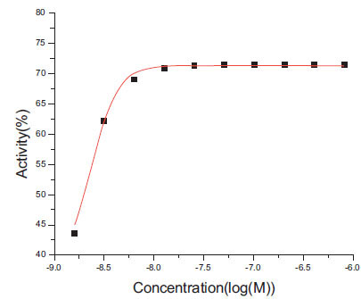 ). For this curve, the actual ymin is -15.9, but the fitted value is 37.5%. The median difference of ymax is 0.36%, and the maximum one is 38.75%. The dose-response curve with the maximum difference is plotted in Fig. (2
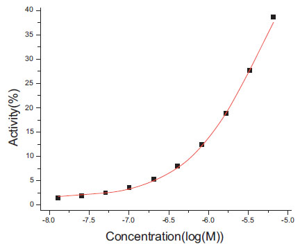 ). For this curve, the actual ymax is 90.75%, but the fitted value is 64.0%. For these a few partial curves, the Grid program apparently has difficulty in reproducing the actual ymin and ymax values. For curves of 20 data points, as expected, the differences between fitted and actual ymin and ymax values are smaller for two reasons. First, more data points add more constraints for and thus reduce the possible space of solutions. Second, most of the 20 data points curves are complete curves.
With increasing noise, the differences between fitted and actual values grow larger. Among the four parameters (EC50, slope, ymin, and ymax), EC50 and ymax are biologically the most important; and here we will focus on these two parameters. For curves of 10 data points, as the number of randomly perturbed data points increases from 0 to 4, correlation coefficient for EC50 decreases from 0.997 to 0.673, 0.612, 0.370, and 0.278; the number of curves with maximum difference of EC50 > 2.0 increases from 0 to 5, 10, 18, and 28; and there are no curves with maximum difference of ymax > 100%. For curves of 20 data points, the results are remarkably better. The correlation coefficients remain > 0.65, and the number of curves with EC50>2.0 only rises from 0 to 1, 6, 9, and 11. Overall, the Grid program is able to recover the actual parameters for most of the simulated data even with 4 of 10 data points randomly perturbed, and the fitted values remain significantly correlated with the actual ones (p < 0.05 with one exception of 0.055).
The Grid program failed to fit 49 curves of 10 data points out of 400 curves with noise. We examined these failed dose-response curves and plot a typical one in Fig. (3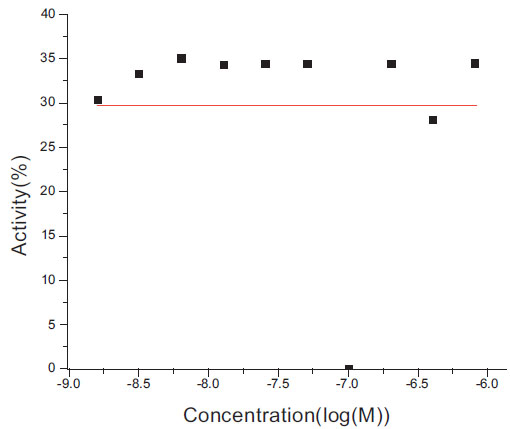 ). This curve has 3 data points randomly perturbed. Apparently, the perturbation disrupted the original curve and made it insignificant.
For recovering the actual parameters of dose-response curves, 20 data points are substantially better than 10 data points. But the Grid program is still able to recover the actual parameters for most of the simulated and partial curves of 10 data points. For high throughput data screening, this is critical. First, 10 data points curves are more economical to generate than 20 data points ones. Second, for HTS, it is difficult to optimize the concentration range to generate a full dose-response curve for compounds of great difference in potency.
3.2. Comparison Between Grid and DRC Program
The fitting results by DRC are given in Table 2. The starting parameters are automatically assigned by DRC. For data without noise, DRC performs better than the Grid program in recovering the actual parameters with only one exception: the maximum difference of ymin for 20 data points curves is 138.35%. In the Grid algorithm, each parameter is sampled at a defined interval. For practical application, the accuracy in the fitted values by Grid algorithm is sufficient. For example, the default sampling interval for EC50 is 0.05, and this corresponds to a difference in concentration by 100.05 or 1.12 times. For drug screening process, two times difference is generally acceptable. From a purely mathematical and numeric point of view, however, the solutions from DRC have better accuracy than the Grid algorithm.
For 10 data points curves with noise, however, DRC’s performance degrade substantially. Out of 16 correlations (four parameters (EC50, slope, ymin and ymax) by four data sets), only three have significant correlation (p<0.05). Some correlation coefficients are even negative. The largest median difference in EC50 is 1.51 or 31 (101.51) times different, and the largest maximum difference is 43.53 or 3x1043 times different. The largest median differences in ymin and ymax are 25.9% and 23.65%, and the largest maximum ones are 1,870% and 1,520%, respectively. As the number of randomly perturbed data points increases from 0 to 4, the correlation coefficient for EC50 decreases from 1.0 to 0.136, -0.042, 0.150, and 0.072; the number of curves with maximum difference of EC50 > 2.0 increases from 0 to 10, 26, 28, and 33; and the number of curves with maximum difference of ymax > 100% increases from 0 to 2, 6, 6, and 5. For curves of 20 data points, the results are better. Out of 16 correlations, most have a significant correlation (p<0.05).
In a word, DRC is very sensitive to noises, it tends to produce biologically unreasonable solutions, and the Grid program is much more robust. One main reason for the Grid program’s robustness is that it effectively has multiple starting points; in fact, it tries all possible starting points in a grid. Using multiple starting points is expected to improve the performance of DRC.
3.3. Comparison Between XLfit Programs with and Without Prefit
XLfit program has the option of prefitting four parameters. The fitting results by XLfit with and without prefit are given in Tables 3 and 4, respectively. The results from prefit are generally worse than those without prefit. For example, for EC50, seven out of the eight correlations (four data sets of 20 data points with noise and four data sets of 10 data points with noise) are significant (p<0.05) without prefit, but only two are significant with prefit. The maximum differences between the fitted and actual values tend to be larger for results with prefit than those without prefit.
3.4. Comparison Between Grid, DRC and XLfit Programs
Like DRC, for data without noise, XLfit performs better in recovering the actual parameters than the Grid program. For data with noise, however, XLfit generally performs worse than DRC. First, the maximum differences between the fitted and actual parameters by XLfit are much larger than those by DRC. Second, even for curves of 20 data points, most of the 16 correlations become insignificant (p>0.05). We tried various options provided by XLfit such as locking a parameter at a prefitted value, but it did not improve.
Comparing with DRC and XLfit programs, the Grid program has two major advantages. The most important one is its robustness and accuracy. The Grid program is able to consistently reproduce the actual values for both complete and partial curves without or with noise. Both DRC and XLfit perform well for data without noise, but they are very sensitive to noise and their performance degrades rapidly with increasing noise. As discussed above, being able to recover actual values of four Hill parameters for partial curves with noise is very important for HTS.
Second, the Grid program is automated and scalable: It does not need to try various starting points in order to achieve good fitting, and it automatically identifies and masks outlier data points. At NCGC, the Grid program is routinely used to fit hundreds of thousands of curves with minimum human interaction. For high quality and high throughput fitting of large number of dose-response curve data, the Grid program has been proven indispensable.
The Grid program’s robustness can be attributed to the very nature of the Grid algorithm. The Grid algorithm searches the best solution of each parameter at a predefined interval in the biologically reasonable domain, it is designed to avoid local minimum trap, and it does not need any starting points. The Grid algorithm does not evaluate any derivatives. The DRC and XLfit programs use first and second order derivatives to find the direction for downward movement. For data of poor quality, the derivatives could be numerically unstable, and the DRC and XLfit programs could be trapped in local minimum to produce unreasonable solutions.
In this study we focus on high throughput fitting of large amount of dose-response data and manual interaction with individual curves is not allowed. For the simulated data with noise, manual interaction, such as trying different starting points and identifying outlier data points, should improve the fitting results for the DRC and XLfit programs. Such manual interaction, however, is time-consuming, subjective and error-prone, and it is not feasible for fitting large number of dose-response data.
3.5. Benchmarking and Practical Application of Grid Program
Exact benchmarking and comparison of speed for the Grid, DRC and XLfit programs is difficult. For processing 500 20 data points dose-response curves, the Grid program took about 200 seconds on Mac Pro with 3GHz Intel Xeon micro processor using the default settings. The 200 seconds include outlier detection, fitting, statistical evaluation, and possible refitting. On the same machine, DRC took 470 seconds. But this comparison is not fair: In the R script for fitting the simulated data, the DRC library was loaded for each dose-response curve; the loading process could take more time than the fitting itself. For XLfit, we imported data into Excel on a windows XP machine and used a macro to perform the curve fitting. Since invoking the macro is a manual process, exact timing is not practical. Excluding manual interactions, the speed of XLfit seems comparable to the Grid program or faster.
As demonstrated in analyzing large amount of dose-response data at NCGC, the Grid program is very productive, robust, and scalable, and it routinely processes hundreds of thousands of dose-response curves with minimum manual intervention. The Grid program has a prescreening module to detect and skip those biologically insignificant curves. For 100,000 7-point dose-response curves, the Grid program is able to accomplish curve fitting, statistical testing, and database transaction within one CPU hour on Linux workstation with 3GHz Intel multi-core Xeon microprocessor. The Grid program supports multiple threads, and it is scalable to millions of dose-response curves.
4. CONCLUSION
The Grid program is robust, automated, and scalable for high throughput analysis of large amount of dose-response data, it consistently reproduces the actual values for both complete and partial curves with or without noise, and it will help in speeding drug development and reducing the cost. For very large data set, it can be indispensible. For data set of small and medium size, the Grid program will enhance the productivity and avoid human errors. The Grid algorithm is also applicable to many other curve fitting problems in biological and medical sciences.
REFERENCES
| [1] | Liu B, Li S, Hu J. Technological advances in high-throughput screening Am J Phamacogenomics 2004; 4: 263-76. |
| [2] | Inglese J, Auld DS, Jadhav A, et al. Quantitative high-throughput screening: A titration-based approach that efficiently identifies biological activities in large chemical libraries Proc Natl Acad Sci USA 2006; 103: 11473-8. |
| [3] | Motulsky HJ. Fitting models to biological data using linear and nonlinear regression: a practical guide to curve fitting In: USA: Oxford University Press 2004. |
| [4] | Motulsky HJ, Ransnas LA. Fitting curves to data using nonlinear regression: a practical and nonmathematical review FASEB J 1987; 1: 365-74. |
| [5] | Levenberg K. A Method for the Solution of Certain Non-Linear Problems in Least Squares Q Appl Math 1994; 2: 164-8. |
| [6] | Ritz C, Streibig JC. Bioassay analysis using R J Stat Softw 2005; 12: 1-22. |
| [7] | R Development Core Team. R: A language and environment for statistical com- puting. R Foundation for Statistical Computing, Vienna, Austria 2005 http://www.R-project.org ISBN 3-900051-07-0 |
| [8] | Hill AV. The possible effects of the aggregation of the molecules of hæmoglobin on its dissociation curves J Physiol 1910; 40: 4-7. |