- Home
- About Journals
-
Information for Authors/ReviewersEditorial Policies
Publication Fee
Publication Cycle - Process Flowchart
Online Manuscript Submission and Tracking System
Publishing Ethics and Rectitude
Authorship
Author Benefits
Reviewer Guidelines
Guest Editor Guidelines
Peer Review Workflow
Quick Track Option
Copyediting Services
Bentham Open Membership
Bentham Open Advisory Board
Archiving Policies
Fabricating and Stating False Information
Post Publication Discussions and Corrections
Editorial Management
Advertise With Us
Funding Agencies
Rate List
Kudos
General FAQs
Special Fee Waivers and Discounts
- Contact
- Help
- About Us
- Search


The Open Cybernetics & Systemics Journal
(Discontinued)
ISSN: 1874-110X ― Volume 12, 2018
Numerical Investigation of Multi-field Coupling Problems on Magneto Hydrodynamics Propulsion by Surface
Zong Kai Liu1, 2, *, Ben Mou Zhou2, Yu Ming Bo1, Yan Ji2, Ya Dong Huang2, Qi Yu3
Abstract
The influence of Multi-field coupling on EMHD (electromagnetic hydrodynamics) propulsion by surface has been numerically investigated in this paper. In former studies, induced item in Lorentz force is usually ignored due to low Reynolds number or weakly conductive fluid. However, for some special environments, this influence of induced item cannot be ignored anymore. Based on navigation model, numerical simulation of EMHD propulsion by surface at Reynolds number 104 are carried out to examine the influence of propulsion effect and flow field characteristic by different magnetic. This result shows that, within a certain range, the efficiency improved with magnetic field intensity, however with its further increase the efficiency decreases, which depends not only on magnetic but also on Reynolds number. Moreover, instead of machine driven, this propulsion scheme offers several advantages over the conventional locked train gear drives, such as noise reducing, less space requirement and so on. This article further explores some of the basic principles of EMHD propulsion and provides a methodology for evaluating the performance of such systems.
Article Information

Identifiers and Pagination:
Year: 2017Volume: 11
First Page: 13
Last Page: 23
Publisher Id: TOCSJ-11-13
DOI: 10.2174/1874110X01711010013
Article History:
Received Date: 05/09/2015Revision Received Date: 04/09/2016
Acceptance Date: 08/09/2016
Electronic publication date: 25/01/2017
Collection year: 2017
open-access license: This is an open access article licensed under the terms of the Creative Commons Attribution-Non-Commercial 4.0 International Public License (CC BY-NC 4.0) (https://creativecommons.org/licenses/by-nc/4.0/legalcode), which permits unrestricted, non-commercial use, distribution and reproduction in any medium, provided the work is properly cited.
* Address correspondence to this author at the Advanced Weapon Launch Collaborative Innovation Center, Nanjing University of Science and Technology, Nanjing University of Science and Technology (Xiao Linwei 200#), Nanjing, JiangSu, China; Tel/Fax: 15105164676; E-mail: kfliukai@126.com
| Open Peer Review Details | |||
|---|---|---|---|
| Manuscript submitted on 05-09-2015 |
Original Manuscript | Numerical Investigation of Multi-field Coupling Problems on Magneto Hydrodynamics Propulsion by Surface | |
1. INTRODUCTION
The design of direct-drive marine engines, ship propellers and micro-space propulsions have reached an advanced stage of development, and only incremental advances in performance may be expected in the future without introduction of new technology or new propulsion concepts. So the EMHD (electromagnetic hydrodynamics) propulsion has achieved more attention in recent years.
If navigation immersed in conductive fluid (seawater, plasma, etc.), electromagnetic force or Lorentz force would be generated by applied electric field and magnetic field around the surface, which could control and propel the surround fluid. Flow control with Lorentz force was first proposed by Rice in 1961, during the following years researchers have developed and applied this methods on ship propulsion [1M.C. Gourdine, "Recent advances in magnetohydro-dynamic propulsion", ARS J., vol. 31, no. 12, pp. 1670-1677, 1961.
[http://dx.doi.org/10.2514/8.5890] , 2S. Molokov, and R. Moreau, Magnetohydrodynamics: Historical Evolution and Trends., Berlin Heidelberg Press: New York, 2007.
[http://dx.doi.org/10.1007/978-1-4020-4833-3] ]. Then a large amount of works have been devoted to study the structure and field distribution of electromagnetic actuators, in weakly conductive fluid. For electrolyte solution like seawater, Lorentz forces provide several attractive approaches in flow control, such as boundary layer control [3K.S. Breuer, J. Park, and C. Henoch, "Actuation and control of a turbulent channel flow using Lorentz forces", Phys. Fluids, vol. 16, pp. 897-907, 2004.
[http://dx.doi.org/10.1063/1.1647142] , 4V. Shatrov, and G. Gerbeth, "Magnetohydrodynamic drag reduction and its efficiency", Phys. Fluids, vol. 19, p. 035109, 2007.
[http://dx.doi.org/10.1063/1.2714077] ], drag reduction [5J. Pang, and K.S. Choi, "Turbulent drag reduction by Lorentz force oscillation", Phys. Fluids, vol. 16, pp. L35-L38, 2004.
[http://dx.doi.org/10.1063/1.1689711] , 6J. Pang, K. Choi, and A. Aessopos, "Control of near-wall turbulence for drag reduction by Spanwise oscillating Lorentz force", In: 2nd AI-AA Flow Control Conference, Oregon: Portland, 2004, p. 28.], lift enhancement [7Y.H. Chen, B.C. Fan, and Z.H. Chen, "Flow pattern and lift evolution of hydrofoil with control of electro-magnetic forces. Science in China Series G: Physics", Mech. Astron., vol. 52, pp. 1364-1374, 2009.
[http://dx.doi.org/10.1007/s11433-009-0172-4] ] as well as noise suppression [8Z. Chen, and N. Aubry, "Closed-loop control of vortex induced vibration", Commun. Nonlinear Sci. Numer. Simul., vol. 10, pp. 287-297, 2005.
[http://dx.doi.org/10.1016/S1007-5704(03)00127-8] ]. Furthermore, Lorentz force has been successfully used in satellite electric propulsion (attitude control and station keeping, etc.) [9L. Garrigues, and P. Coche, "Electric propulsion: comparisons between different concepts", Plasma Phys. Contr. Fusion, vol. 53, p. 124011, 2011.
[http://dx.doi.org/10.1088/0741-3335/53/12/124011] -11S. Tsujii, M. Bando, and H. Yamakawa, "Spacecraft formation flying dynamics and control using the geomagnetic Lorentz force", Control, and Dynamics., vol. 36, pp. 136-148, 2013.
[http://dx.doi.org/10.2514/1.57060] ], in this way plasma or charged particle can be accelerated and injected to adjust satellite attitude. So if the navigation is covered with body-fitted electromagnetic actuators, Lorentz force would be generated and propelled the surround fluid, this is the basic principle of EMHD propulsion by surface. EMHD propulsion is a kind of static electric magnetic propulsion system, which had attracted the attention of several inventors over the past several years [12Z.K. Liu, B.M. Zhou, H.X. Liu, and Z.G. Liu, "The analysis of effects and theories for electromagnetic hydrodynamics propulsion by surface", Wuli Xuebao, vol. 60, pp. 84701-084701, 2011., 13Z.K. Liu, J.L. Gu, and B.M. Zhou, "Investigation of electromagnetic hydrodynamics propulsion and vector control by surfaces based on a rotational navigation body", Wuli Xuebao, vol. 63, pp. 74704-074704, 2014.]. The main reason for this attraction has been the seemingly elegant operating principle using no moving parts. Proposed applications include the silent propulsion of naval submarines, the use in high-speed cargo submarines, and the propulsion of future high-speed surface ships without the danger of cavitation.
During the EMHD propulsion, the presence of an external magnetic field B in an electrically conducting flow gives birth to an induced magnetic field and induced electrical currents. When the magnetic Reynolds number Re is much smaller than 1, as in small liquid metal experiments, the induced magnetic field is negligible, but not the induced currents and the total magnetic field is the imposed one [14P.A. Davidson, An Introduction to Magnetohydrodynamics., Cambridge University Press: UK, 2001.
[http://dx.doi.org/10.1017/CBO9780511626333] ]. The Lorentz force generated by the interaction between the magnetic field and the induced currents tends to damp velocity variations along the streamlines [15J.L. Sommeria, and R. Moreau, "Why, how, and when, MHD turbulence becomes two-dimensional", J. Fluid Mech., vol. 118, pp. 507-518, 1982.
[http://dx.doi.org/10.1017/S0022112082001177] ]. EMHD propulsion by surface would also be applied widely, such as high-speed aircraft flight in ionosphere or outer space. For some special circumstances, in order to achieve better propulsion effects the environment parameters such as the electrical conductivity and permeability could be improved by release special medium (such as plasma). The recently dramatic developments in high-temperature superconducting materials and the successful operation of a large and sophisticated magnet system at Laboratory now make it desirable to reconsider EMHD propulsion. Under these conditions, the disturbance of induced item to propulsion effects must be considered. So in this paper numerical investigations have been conducted on the basic of this special environment.
2. THE BASIC MODEL AND NUMERICAL METHOD
2.1. The Basic Model
Fig. (1) is schematic of the navigation model. The navigation leading edge point is located at the origin coordinate and is designed to generate surface tangential Lorentz force along the positive x-direction. The model length is L, semi-circular head radius R=0.06L, cylindrical navigation body length L0=0.69L, and tail cone length L1=0.25L. The cylindrical surface of navigation model is covered by propulsion cells as shown in Fig. (1), by which Lorentz force can be generated. The propulsion cell is a stripwise arrangement of flush mounted electrodes and permanent magnets of alternating polarity and magnetization (N, +, S, −). The Lorentz force acting tangential to the surface can either assist or oppose the flow as Fig. (1) shows:
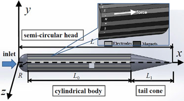 |
Fig. (1) Schematic of the navigation model. |
Introduce b as the induced magnetic field and B as the total magnetic field. Based on the Ohm’s Law and Maxwell equation, the magnetic induction equation can be obtained as follows
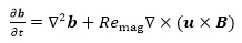 |
(1) |
The is magnetic Reynolds number, which is typically low for weakly conducting fluid, hence the induced item can be neglected and equation (1) does not have to be solved over time. For Re=100 flows several typical engineering magnetic Reynolds numbers are listed that salt water molten steel 1. When the much smaller than 1, as in small liquid metal experiments, the induced magnetic field is negligible, but not the induced currents, and the total magnetic field is the imposed one [16V. Dousset, and A. Pothérat, "Numerical simulations of a cylinder wake under a strong axial magnetic field", Phys. Fluids, vol. 20, p. 017104, 2008.
[http://dx.doi.org/10.1063/1.2831153] ]. The interaction between the induced currents and the magnetic field generates Lorentz forces that tend to damp velocity variations along the streamlines. So for certain specific control mode or application environment, the influence of magnetic induced item on total force cannot be ignored. Based on this phenomenon, the propulsive characteristic under certain hypothetical environment is numerical investigated in this paper.
2.2. Basic Control Equations and the Numerical Methods
The non-dimensional Navier-Stokes equations for the incompressible flow are given below.
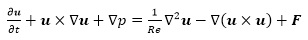 |
(2) |
 |
(3) |
All lengths and velocities are non-dimensionalized with respect to the navigation chord L and U∞. And the electric field and magnetic field are non-dimensionalized by characteristic magnetic field and electric field.
In equation (2) F is the source item of governing equation denotes the external body force. In EMHD problem, F is the Lorentz force,which can be written as:
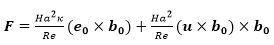 |
(4) |
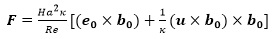 |
(5) |
Where
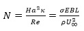
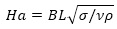 is the Hartmann number denotes the ratio of Lorentz force to viscous force, Reynolds number Re = ρLU∞/v and κ = E / U∞ is the ratio of applied electric field to induced electric field. The σ, ρ and ν are the medium’s electric conductivity, density and viscosity, respectively. B and E are the characteristic scale for magnetic field and electric field, respectively.. In the following paper, we use N as interaction parameters denotes the ratio of Lorentz force to inertia.
 |
(6) |
The numerical analysis model is shown in Fig. (1). The axis of navigation overlaps with x axis and the inlet flow along positive direction of x axis. If the interaction parameter N and the Hartmann number Ha are large, the flow is invariant along the magnetic lines, expect in the vicinity of walls that intersect them. In this region, viscous forces maintain strong velocity gradients and the so-called Hartmann layer develops. The resulting flow, made of Hartmann layers and a core flow where the velocity is constant along the magnetic field lines, is called quasi-two-dimensional (quasi-2D). So on the assumption of infinite long electrodes and magnets in the streamwise direction (edge effects are neglected) and the inlet flow (x-direction velocity) is dominant, the influence of u velocity to induced item should be mainly considered and the other perturbations (y and z direction velocities) could be ignored. Thus the distributions of electric field and magnetic field can be assumed parallel to yz plane. Furthermore, the components of electromagnetic vector and magnetic field vector in y and z directions are not zero. By this way, Lorentz force along the positive direction of x axis is generated by the mutual interaction of electric field and magnetic field. Accordingly, the field distributions could be calculated by Maxwell equations [17T.W. Berger, J. Kim, and C. Lee, "Turbulent boundary layer control utilizing the Lorentz force", Phys. Fluids, vol. 12, pp. 631-649, 2000.
[http://dx.doi.org/10.1063/1.870270] -20H. Zhang, B.C. Fan, and Z.H. Chen, "Control approaches for a cylinder wake by electromagnetic force", Fluid Dyn. Res., vol. 41, p. 045507, 2009.
[http://dx.doi.org/10.1088/0169-5983/41/4/045507] ].
According to Lenz’s law, induced electromotive force always gives rise to current whose magnetic field opposes the original change in magnetic flux. So the Lorentz force is always inhibited or weakened due to the action of induced item. For this case, the changing of total force is depends no longer only on the wall distance, but also on the time and velocity in each node.
In this numerical simulation, the compute region is divided into many small tetrahedron elements firstly. These elements as well as their four nodes are numbered by a set of integral values. 4×M array n(i,e),i = 1,2,3,4;e = 1,2,3…M (where M denotes the total number of tetrahedron element) is used to store the information of elements and nodes. Secondly, the relevant location relationship between elements and notes are stored with corresponding matrix. Finally, based on the governing equations the corresponding velocity pressure interpolation function is calculated. In the process of simulation, linear interpolation is utilized as the pressure interpolation, due to the fact that the momentum transfer caused by pressure is first order. While the viscosity fluid transfer caused by strain rate is second order, hence the quadratic approximation function method is employed as the speed interpolation [21H.F. Joel, Milovan P Computational Methods for Fluid Dynamics., Springer-Verlag Press Berlin: Berlin, 2002, pp. 164-206.-23J.N. Reddy, and D.K. Gartling, The Finite Element Method in Heat Transfer and Fluid Dynamics., CRC Press: USA, 2010.].
In order to verify the validity of the algorithm, the three dimensional infinite long cylindrical flow are simulated and compared with previous research results. The cylinder diameter of calculation model denotes D, its length is 10D, Re=100. The drag coefficient, lift coefficient, Strouhal numbers are defined, respectively
 |
where SD = D × 10D is cylindrical cross sectional area, fD is vortex shedding frequency. Kim J and Kim D [24J. Kim, D. Kim, and H. Choi, "An immersed-boundary finite-volume method for simulations of flow in complex geometries", J. Comput. Phys., vol. 171, no. 1, pp. 132-150, 2001.
[http://dx.doi.org/10.1006/jcph.2001.6778] ] has researched the flow around circular cylinders at Re=100. They measured that the moment fluctuation range could stabilize to ±0.328 and Cd ≈ 1.33, St ≈ 0.165. Fig. (2) is the histories of lift coefficient and drag coefficient. The figure shows that Cl changes within ±0.312, Cd ≈ 1.31, St ≈ 0.16° Thus, compared with the previous experiment can be seen that this algorithm in solving this problem is of good precision.
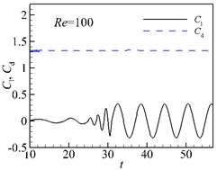 |
Fig. (2) Cylindrical flow around numerical algorithm validation (Re = 100). |
3. THE INFLUENCE OF MAGNETIC FIELD ON FLOW FIELD AROUND THE NAVIGATION
To gain some insight into the effect of magnetic induction intensity to propulsion character, numerical simulations have been conducted at Re= 1 × 10⁴ with three different interaction parameters. 1. N=40, 1⁄κ=8, 2. N=160, 1⁄κ=2, 3. N=240, 1⁄κ=4/3. The selecting of these parameters is to reflect the influence of three different magnetic intensities to propulsive characteristics. During this simulation, the electric field intensity is kept constant.
Fig. (3) shows the distributions of velocity amplitude isosurface range from 5.5 to 6.5, which are slightly larger than U∞=5. For unforced case, t=1.8 as Fig. (3a) shows that velocity isosurface just appears around the leading edge. However, when the force applied the isosurface near the leading edge as well as the navigation body surface is extended. The largest velocity isosurface appears in Fig. (3c) at t=3.8, and then the Fig. (3b and d). It could be concluded that the change of propulsion force with magnetic field intensity presents nonlinear characters. In order to reveal this influence, further analysis will be listed in the following paper.
In order to display the velocity changes better with wall normal distance, a spherical surface is defined as Fig. (4) shows with center (L/2, 0, 0) and radius 2R. The distributions of fluid field over this surface would be mainly analyzed in the following paper.
Fig. (5a) is the u velocity distribution on the spherical surface at t=3.8 (force stability action time). Fig. (5b) is the curve of u velocity along wall normal distance from the center location, where Fig. (5a) shows that on the spherical surface relatively low speed boundary layer still appears near the surface, due to the fluid viscous. With wall distance increasing red high speed region appears, but flow velocity on the further region gradually attenuates to U∞. The high velocity range on the left side of spherical surface is narrower than the rightbecause the downstream fluid continuously obtained the kinetic energy of Lorentz force, which leads to an increase of near wall fluid velocity. It could also be seen from Fig. (5b), that a low speed. Meanwhile, u velocity is increasing away from the surface with the action of Lorentz force, and the maximum velocity 5.3 appears within the high speed range corresponding to the high speed red area shown in Fig. (5a).
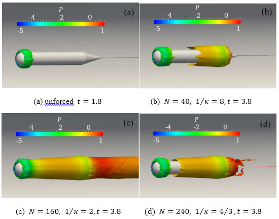 |
Fig. (3) The distributions of velocity isosurface (5.5~6.5). |
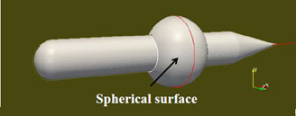 |
Fig. (4) Schematic of the spherical surface. |
In order to offer more detail interpretations of velocity distribution in Fig. (5), Fig. (6) is drawn to display the distribution curves of Lorentz force and its each component along wall normal distance, at t = 3.8 (Force in Fig. (5a) denotes the total Lorentz force, Force1 is the conducting item intensity, Force2 denotes the induced item intensity and Force=Force1−Force2). The force action range. And the distribution of Force1 is related only to the intensity of electric field and magnetic field, which does not change with the fluid flow velocity. The fluid around the surface is of lower u velocity, so force intensity is relatively small, about 0.5. However, with wall distance increasing, Force2 reaches to the maximum 3.2 at d1/R ≈ 0.25. The u velocity intends to U∞ in farther distance, but Force2 decreases to zero due to the attenuation of total force along wall normal distance. Fig. (6c) is the distribution curve of Lorentz force. Owing to the negative effect of induced items on Lorentz force, it could befound that the total force decreases. By comparing Fig. (6a and c), we could find that there is no remarkable difference between the distribution curves of Force1 and Force except for their gradients.
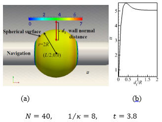 |
Fig. (5) The flow velocity distribution on spherical surface, and changes curve along the normal distance. |
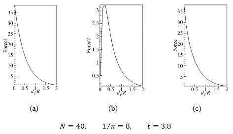 |
Fig. (6) Distribution curves of the Lorentz force and its each component along the wall normal distance. |
Fig. (7a) is the u velocity distribution on the spherical surface at t = 3.8. Fig. (7b) is the curve of u velocity along wall normal distance from the center location, whereUnder the action of Lorentz force, high speed fluid is appeared and surrounded the navigation. Meanwhile, the fluid velocity is increased under this force control, so as illustrated in Fig. (7b) the red high velocity range is extended slightly larger than the former case (N = 40, 1⁄κ = 8, t = 3.8).
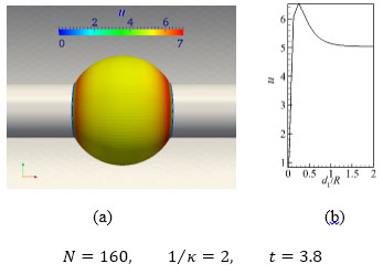 |
Fig. (7) The flow velocity distribution on spherical surface, and changes curve along the normal distance. |
As Fig. (7b) shows the near wall (0.1 < d1/R < 1.6) fluid is of larger velocity than U∞. That the u velocity along the wall normal reaches to the maximum 6.35. Moreover, the low velocity (u < 5) range is constantly contracted to 0 < d1/R < 0.1. This illustrates that when keeping the electric field intensity constant, the increase of magnetic induction intensity within a certain range can promote the Lorentz force.
Fig. (8) is the distribution curves of Lorentz force and its each component, t=3.8. As the Fig. (8a ) shows Force1 intends to decay exponentially with wall distance. The maximum of Force1 appears at about 160, near the surface, but then decay to zero gradually with wall distance increases. The Fig. (8b) displays that when Force2 intends to 12, but with the wall distance increasing the peak 74 of Force2 occurred at approximately way from the surface, and then decay to zero gradually.
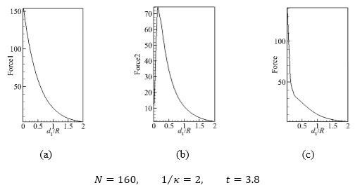 |
Fig. (8) Distribution curves of the Lorentz force and its each component along the wall normal distance. |
Near wall, the flow velocity is rather low even N is bigger; but the product of N and u velocity is also very small. Compare Fig. (8c) with (8a) it could note that Force in range of 0 < d1/R < 1 has more sharply attenuation gradient, so Force1 ≈ 55 at d1/R = 0.5, but Force ≈ 27, which is mainly due to the inhibition of magnetic induced intensity.
Fig. (9a) is the u velocity distribution on the spherical surface at t = 3.8 (Lorentz force stability action time). Fig. (9b) is the curve of u velocity along wall normal distance from the center location of navigation surface,. It could be found that the total force intensity decreases with further increasing of η. Accordingly, u velocity of near wall fluid is decreased and the red high velocity range (0.12 < d1/R < 1.2, u > 5) is contracted. For this case, the maximum of u velocity is 5.95 larger than the first case but smaller than the second one, which causes the boundary layer thickness (0 < d1/R < 0.12, u < 5) narrower than the former.
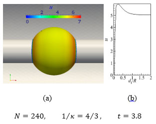 |
Fig. (9) The flow velocity distribution on spherical surface, and change curve along the normal distance. |
Fig. (10) is the distribution curves of Lorentz force and its each component, t=3.8. As this figure shows, Force1 decreases exponentially with wall normal distance. So near the surface, Force1 appears the maximum about 160, but then decreases to zero gradually with the increase of wall distance. As shown in Fig. (10b) the induction of electromagnetic force Force2 near the surface is almost zero, which is caused by the boundary layer. However, the flow velocity increases with the increase of wall normal distance and reaches to the maximum 160 at 0.15. Comparing with Force1, the proportion of induced item Force2 to total force increases gradually. The Fig. (10c) is the distribution curve of Force. The intensity of induced item is larger near the surface, which leads to a sharply decrease of Force in. Then with the increasing of wall distance the gradient of Force decrease intends to slowly. In fact, the above investigations suggest that the increasing of η in center range could promote the total Lorentz force. However, when the percent of induced item exceeds a certain value, the total force will decrease with the further increase of induced item.
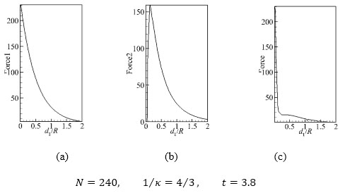 |
Fig. (10) Distribution curves of the Lorentz force and its each component along the wall normal distance. |
4. THE FLUID DYNAMICS CHARACTER OF NAVIGATION
The force in each direction would be mainly analyzed based on flow fluid structure, in the following paper. We set ft = fprx + fshx the total force, where fprx and fshx are the pressure force and shear force in x-direction, respectively; while florx and florx1 denote the total Lorentz force and applied item, respectively. The force histories are recorded from flow stable time t=0.5, and the force action time range is from t=2 to 4.
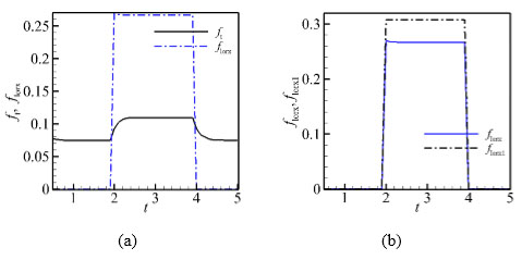 |
Fig. (11) Time histories of each forces (N = 40, 1/κ = 1, case1). |
Fig. (11a and b) are time histories of ft, florx and florx, florx1, respectively. As Fig. (11a) shows ft intends to 0.075 without force control but then increases sharply to 0.11 since t = 2. During this time, it could be found that florx increases from 0 to 0.27 (at t=2.05) and then decreases slightly to 0.266. This is due to that while the Lorentz force is applied, the velocity u increases from zero, which brings about a continue increase influence of induced item on total Lorentz force. Finally, this influence intends to stability. As Fig. (11b) shows, a peak value of florx appears at the beginning of force applied. But the applied item florx1 keeps constant at about 0.31, which is larger than the total Lorentz force ft.
Fig. (12a and b) are time histories of ft, florx and florx, florx1, respectively. For this case, with the increase of magnetic field, the influence of induced item is expanded.
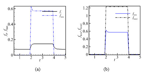 |
Fig. (12) Time histories of each forces (N = 160, 1/κ = 2, case2). |
The Fig. (12a) displays that florx jumps to peak value 0.64 while the force applied but then decreases slowly to 0.56 at about t=2.3. This change is similar to the former case, but the stable value of florx is 0.56 (N = 160, 1/κ = 2) larger than 0.266 (N = 40, 1/κ = 8). The increase of magnetic field leads to a significant rise in fluid velocity and drags force thus ft increases and becomes stabilized at about 0.15. Compare Fig. (12b) with (11b), it could be found that the applied item florx1 ≈ 1.24 (N = 160, 1/κ = 2) keeps constant over t = 2-4, whichis about four times larger than florx1t ≈ 0.31(N = 40, 1/κ = 8).
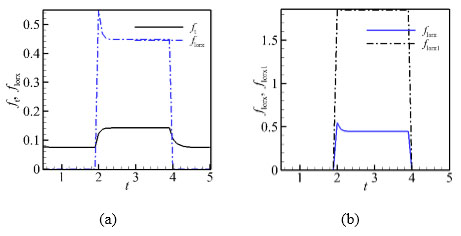 |
Fig. (13) Time histories of each forces (N = 240, 1/κ = 4/3, case3). |
It can be seen in the Fig. (13) that, with further increase of magnetic field, more significant inhibition effect for navigation propulsion is observed. So comparing with the former two cases florx reaches to the maximum 0.56 and then falls sharply to a plateau 0.44 less than 0.64 (case 2). Accordingly, ft approximately stabilizes at 0.14 also less than the former cases and the difference between florx ≈ 0.44 and florx1 ≈ 1.92 is enlarged.
Then we introduce Cpro as thrust coefficient of navigation
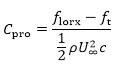 |
The Cpro for the three cases at Re = 1 × 10⁴ are listed in Table 1. It could be found that the Cpro ≈ 0.0328 of case 2, is 60.97% and 26.83% larger than that of case1 and case 3, respectively.
CONCLUSION
For larger Reynolds number or magnetic Reynolds number environment, the influence of induced item on navigation surface propulsion effects could not be ignored anymore. In this paper, based on navigation model, the influence of three different magnetic intensities (keep the electric field intensity constant) on flow field characteristic and propulsion effects have been analyzed. These conclusions reveal that while keeps the electric field constant, the thrust coefficient of navigation rises with the increasing of magnetic field at first but then drops more quickly. The change of thrust coefficient with magnetic field intensity also presents a nonlinear character, which depends not only on magnetic field but also on the Re and Remag.
CONFLICT OF INTEREST
The authors confirm that this article content has no conflict of interest.
ACKNOWLEDGEMENTS
This work is supported by the postdoctoral funds of Jiangsu province, NO.1401123C, Jiangsu province youth fund, NO.BK20140792 and the postdoctoral funds of china, NO.2015M571755. Nanjing university of science and technology independent scientific research funds, NO.30915011336.
REFERENCES
| [1] | M.C. Gourdine, "Recent advances in magnetohydro-dynamic propulsion", ARS J., vol. 31, no. 12, pp. 1670-1677, 1961. [http://dx.doi.org/10.2514/8.5890] |
| [2] | S. Molokov, and R. Moreau, Magnetohydrodynamics: Historical Evolution and Trends., Berlin Heidelberg Press: New York, 2007. [http://dx.doi.org/10.1007/978-1-4020-4833-3] |
| [3] | K.S. Breuer, J. Park, and C. Henoch, "Actuation and control of a turbulent channel flow using Lorentz forces", Phys. Fluids, vol. 16, pp. 897-907, 2004. [http://dx.doi.org/10.1063/1.1647142] |
| [4] | V. Shatrov, and G. Gerbeth, "Magnetohydrodynamic drag reduction and its efficiency", Phys. Fluids, vol. 19, p. 035109, 2007. [http://dx.doi.org/10.1063/1.2714077] |
| [5] | J. Pang, and K.S. Choi, "Turbulent drag reduction by Lorentz force oscillation", Phys. Fluids, vol. 16, pp. L35-L38, 2004. [http://dx.doi.org/10.1063/1.1689711] |
| [6] | J. Pang, K. Choi, and A. Aessopos, "Control of near-wall turbulence for drag reduction by Spanwise oscillating Lorentz force", In: 2nd AI-AA Flow Control Conference, Oregon: Portland, 2004, p. 28. |
| [7] | Y.H. Chen, B.C. Fan, and Z.H. Chen, "Flow pattern and lift evolution of hydrofoil with control of electro-magnetic forces. Science in China Series G: Physics", Mech. Astron., vol. 52, pp. 1364-1374, 2009. [http://dx.doi.org/10.1007/s11433-009-0172-4] |
| [8] | Z. Chen, and N. Aubry, "Closed-loop control of vortex induced vibration", Commun. Nonlinear Sci. Numer. Simul., vol. 10, pp. 287-297, 2005. [http://dx.doi.org/10.1016/S1007-5704(03)00127-8] |
| [9] | L. Garrigues, and P. Coche, "Electric propulsion: comparisons between different concepts", Plasma Phys. Contr. Fusion, vol. 53, p. 124011, 2011. [http://dx.doi.org/10.1088/0741-3335/53/12/124011] |
| [10] | K.D. Kumar, and A.M. Zou, "A novel single thruster control strategy for spacecraft attitude stabilization", Acta Astronaut., vol. 86, pp. 55-67, 2013. [http://dx.doi.org/10.1016/j.actaastro.2012.12.018] |
| [11] | S. Tsujii, M. Bando, and H. Yamakawa, "Spacecraft formation flying dynamics and control using the geomagnetic Lorentz force", Control, and Dynamics., vol. 36, pp. 136-148, 2013. [http://dx.doi.org/10.2514/1.57060] |
| [12] | Z.K. Liu, B.M. Zhou, H.X. Liu, and Z.G. Liu, "The analysis of effects and theories for electromagnetic hydrodynamics propulsion by surface", Wuli Xuebao, vol. 60, pp. 84701-084701, 2011. |
| [13] | Z.K. Liu, J.L. Gu, and B.M. Zhou, "Investigation of electromagnetic hydrodynamics propulsion and vector control by surfaces based on a rotational navigation body", Wuli Xuebao, vol. 63, pp. 74704-074704, 2014. |
| [14] | P.A. Davidson, An Introduction to Magnetohydrodynamics., Cambridge University Press: UK, 2001. [http://dx.doi.org/10.1017/CBO9780511626333] |
| [15] | J.L. Sommeria, and R. Moreau, "Why, how, and when, MHD turbulence becomes two-dimensional", J. Fluid Mech., vol. 118, pp. 507-518, 1982. [http://dx.doi.org/10.1017/S0022112082001177] |
| [16] | V. Dousset, and A. Pothérat, "Numerical simulations of a cylinder wake under a strong axial magnetic field", Phys. Fluids, vol. 20, p. 017104, 2008. [http://dx.doi.org/10.1063/1.2831153] |
| [17] | T.W. Berger, J. Kim, and C. Lee, "Turbulent boundary layer control utilizing the Lorentz force", Phys. Fluids, vol. 12, pp. 631-649, 2000. [http://dx.doi.org/10.1063/1.870270] |
| [18] | O. Posdziech, and R. Grundmann, "Electromagnetic control of seawater flow around circular cylinders", Eur. J. Mech. BFluids, vol. 20, pp. 255-274, 2001. [http://dx.doi.org/10.1016/S0997-7546(00)01111-0] |
| [19] | H. Zhang, B.C. Fan, and Z.H. Chen, "Open-loop and optimal control of cylinder wake via electromagnetic fields", Chin. Sci. Bull., vol. 53, pp. 2946-2952, 2008. |
| [20] | H. Zhang, B.C. Fan, and Z.H. Chen, "Control approaches for a cylinder wake by electromagnetic force", Fluid Dyn. Res., vol. 41, p. 045507, 2009. [http://dx.doi.org/10.1088/0169-5983/41/4/045507] |
| [21] | H.F. Joel, Milovan P Computational Methods for Fluid Dynamics., Springer-Verlag Press Berlin: Berlin, 2002, pp. 164-206. |
| [22] | H.K. Versteeg, and W. Malalasekera, An Introduction to Computational Fluid Dynamics: The Finite Volume Method., Pearson Education: USA, 2007. |
| [23] | J.N. Reddy, and D.K. Gartling, The Finite Element Method in Heat Transfer and Fluid Dynamics., CRC Press: USA, 2010. |
| [24] | J. Kim, D. Kim, and H. Choi, "An immersed-boundary finite-volume method for simulations of flow in complex geometries", J. Comput. Phys., vol. 171, no. 1, pp. 132-150, 2001. [http://dx.doi.org/10.1006/jcph.2001.6778] |