- Home
- About Journals
-
Information for Authors/ReviewersEditorial Policies
Publication Fee
Publication Cycle - Process Flowchart
Online Manuscript Submission and Tracking System
Publishing Ethics and Rectitude
Authorship
Author Benefits
Reviewer Guidelines
Guest Editor Guidelines
Peer Review Workflow
Quick Track Option
Copyediting Services
Bentham Open Membership
Bentham Open Advisory Board
Archiving Policies
Fabricating and Stating False Information
Post Publication Discussions and Corrections
Editorial Management
Advertise With Us
Funding Agencies
Rate List
Kudos
General FAQs
Special Fee Waivers and Discounts
- Contact
- Help
- About Us
- Search


The Open Mechanical Engineering Journal
(Discontinued)
ISSN: 1874-155X ― Volume 14, 2020
An Alternate View of Dimensional Homogeneity, and Its Impact on Engineering Science
Eugene F. Adiutori*
Abstract
Aims:
This article proposes an alternate view of dimensional homogeneity that greatly simplifies the solution of nonlinear engineering problems.
Background:
The conventional view of dimensional homogeneity is generally credited to Fourier (1822).
Objectives:
The objectives of this article are to describe the alternate view of dimensional homogeneity and to demonstrate its application to practical engineering problems.
Methods:
By presenting the solution of several nonlinear engineering problems, this article compares solutions based on the alternate view of dimensional homogeneity with solutions based on the conventional view.
Results:
Example problems demonstrate that nonlinear engineering problems are much easier to solve if the solutions are based on the alternate view of dimensional homogeneity rather than the conventional view. The relative simplicity results because the alternate view of dimensional homogeneity reduces the number of variables in nonlinear problems.
Conclusion:
The widely accepted view of dimensional homogeneity should be replaced by the alternate view because the solution of nonlinear engineering problems is greatly simplified.
Article Information
Identifiers and Pagination:
Year: 2018Volume: 12
First Page: 164
Last Page: 174
Publisher Id: TOMEJ-12-164
DOI: 10.2174/1874155X01812010164
Article History:
Received Date: 21/6/2018Revision Received Date: 18/7/2018
Acceptance Date: 27/7/2018
Electronic publication date: 31/08/2018
Collection year: 2018
open-access license: This is an open access article distributed under the terms of the Creative Commons Attribution 4.0 International Public License (CC-BY 4.0), a copy of which is available at: (https://creativecommons.org/licenses/by/4.0/legalcode). This license permits unrestricted use, distribution, and reproduction in any medium, provided the original author and source are credited.
* Address correspondence to this author at the Ventuno Press, 1094 Sixth Lane N., Naples, Florida 34102, USA; Tel: 1-239-537-4107; E-mail: efadiutori@aol.com
| Open Peer Review Details | |||
|---|---|---|---|
| Manuscript submitted on 21-6-2018 |
Original Manuscript | An Alternate View of Dimensional Homogeneity, and Its Impact on Engineering Science | |
1. INTRODUCTION
The alternate view of dimensional homogeneity described herein is founded on the axiom:
Different things cannot be related. Therefore, equations cannot describe how different things are related.
Equations cannot describe how ducks are related to pencils, how trees are related to bicycles, how stress is related to strain, how heat flux is related to temperature difference, etc.
Equations can oftentimes describe how the numerical values of different things are related-how the numerical value of stress is related to the numerical value of strain, how the numerical value of heat flux is related to the numerical value of temperature difference, etc.
In the alternate view of dimensional homogeneity:
- Parameter symbols represent numerical value but not dimension.
- Equations are inherently dimensionless and dimensionally homogeneous.
- Equations describe how numerical values are related. If an equation is quantitative, the dimension units that underlie symbols must be specified in an accompanying nomenclature.
- Parameters such as material modulus and heat transfer coefficient are not required for dimensional homogeneity, and they are abandoned.
- The solution of nonlinear problems is greatly simplified because abandonment of parameters such as material modulus and heat transfer coefficient reduces the number of variables.
This article describes how the alternate view of dimensional homogeneity impacts engineering science, and demonstrates how to solve engineering problems in a dimensionally homogeneous way without using parameters such as heat transfer coefficient and material modulus.
2. THE HISTORY OF DIMENSIONAL HOMOGENEITY
For more than 2000 years--from the time of Aristotle until early in the nineteenth century-scientists and engineers globally agreed that, with one exception, dimensioned parameters cannot be added, subtracted, multiplied, or divided. The one exception is that a dimensioned parameter can be divided by the same dimensioned parameter. For example, the number of feet can be divided by the number of feet, and the number of seconds can be divided by the number of seconds, but the number of feet cannot be divided by the number of seconds.
The following verbal equation by Galileo [1 Galileo, 1638, Two New Sciences, P. 152, translation by Stillman Drake, published 1974 by The University of Wisconsin Press.] is typical. Note that the equation is dimensionless and dimensionally homogeneous because it consists of speed/speed, time/time, and (space run through)/(space run through).
“If two moveables are carried in equable motion, the ratio of their speeds will be compounded from the ratio of spaces run through and from the inverse ratio of times”.
A proportion was often used to describe the relationship between two parameters because a proportion would not require the addition, subtraction, multiplication, or division of dimensioned parameters. For example, Newton’s [2 Newton, I., The Principia, 1726, 3rd edition, translation by Cohen, I. B. and Whitman, A. M., 1999, P. 460, University of California Press.] second law of motion is not Eq. (1). Newton and his contemporaries would have considered Eq. (1) irrational because it requires that dimensioned parameter “m” be multiplied by dimensioned parameter “a”.
 |
(1) |
Newton’s second law of motion as published in Newton [2 Newton, I., The Principia, 1726, 3rd edition, translation by Cohen, I. B. and Whitman, A. M., 1999, P. 460, University of California Press.] is the proportion
A change in motion is proportional to the motive force impressed and takes place along the straight line in which that force is impressed.
Symbolically, Newton’s second law by Newton is Proportion (2).
 |
(2) |
Fourier [3 Fourier, J., 1822, The Analytical Theory of Heat, Article 160, 1955 Dover edition of the 1878 English translation, The University Press.] had a very different view of dimensional homogeneity. In his view:
- Dimensioned parameters can be multiplied and divided.
- Dimensioned parameters cannot be added or subtracted.
- every undetermined magnitude or constant has one dimension proper to itself.
Fourier concluded that Proportion (3) correlated his data. But he did not want a proportion. He wanted a dimensionally homogeneous equation.
 |
(3) |
Transforming Proportion (3) into an equation results in Eq. (4). Note that Eq. (4) is not dimensionally homogeneous because “c” is dimensionless.
 |
(4) |
Fourier recognized that he could make Eq. (4) dimensionally homogeneous only if he could rationally assign the required dimensions to pure number “c”. That is why he stated that a constant in a parametric equation “has one dimension proper to itself”. This statement made it seem rational to assign the required dimensions to pure number “c”, which Fourier did, thereby transforming pure number “c” into dimensioned parameter h, and transforming dimensionally inhomogeneous Eq. (4) into dimensionally homogeneous Eq. (5a)1.
 |
(5a) |
Note that Eq. (5a) requires that dimensioned parameter h be multiplied by dimensioned parameter ΔT. Fourier offered no proof that it is rational to multiply dimensioned parameters, even though it was a revolutionary change from the view held by world-class scientists and engineers for more than 2000 years. The only “proof” given by Fourier is the claim that his view of dimensional homogeneity “is the equivalent of the fundamental lemmas (axioms) which the Greeks have left us without proof”.
Fourier did not present the lemmas in his nearly 500-page treatise, nor did he cite a reference to them. Presumably, his contemporaries accepted his view of dimensional homogeneity without proof because he solved numerous practical problems that his contemporaries were unable to solve.
Although Fourier is generally credited with the current view of dimensional homogeneity, it is important to note that the current view differs from Fourier’s view in a fundamental and very important way. Langhaar [4 Langhaar, H. L., 1951, Dimensional Analysis and Theory of Models, P. 13, John Wiley & Sons.] states:
“Dimensions must not be assigned to numbers, for then any equation could be regarded as dimensionally homogeneous”.
Therefore, parameters such as h, E, and R should be abandoned because they were created by assigning dimensions to numbers, in violation of the current view that “dimensions must not be assigned to numbers, for then any equation could be regarded as dimensionally homogeneous”.
3. THE MEANING OF ENGINEERING LAWS
When Eq. (5a) was conceived by Fourier, it was an equation because it described behavior, and it was a law because it always applied. It stated that, if heat transfer is by steady-state forced convection to atmospheric air, q is always proportional to ΔT, and h is always a proportionality constant.
Sometime near the beginning of the twentieth century, Eq. (5a) ceased to be an equation, and became a definition. Bird, Stewart, and Lightfoot [5 Bird, Stewart, and Lightfoot, 1960, Transport Phenomena, P. 391, John Wiley and Sons, Inc.] and Bejan [6 Bejan, Adrian, 2013, Convection Heat Transfer, 4th edition, P. 32, John Wiley and Sons, Inc.
[http://dx.doi.org/10.1002/9781118671627] ] state that Eq. (5a) is “the defining equation for h”. Note the following:
- Based on generally accepted mathematical terminology, Eq. (5a) is an equation that describes a proportional relationship between q and ΔT, and h is a proportionality constant.
- Since sometime near the beginning of the twentieth century, Eq. (5a) has not been an equation because it does not describe the relationship between q and ΔT.
- Although Eq. (5a) is often referred to as a “law”, it cannot be a law because it is not an equation.
-
Eq. (5a) is a definition in the form of an equation. It defines h to be identical to and interchangeable with q/ΔT. Consequently, Eqs. (5a) and (5b) are identical.
-
(5b)
-
1 Although Eq. (5a) is generally referred to as “Newton’s law of cooling”, Adiutori [7 Adiutori, E. F., 1974, “The New Heat Transfer”, pp. 1-14, 1-15, Ventuno Press. and 8 Adiutori, E. F., 1990, “Origins of the Heat Transfer Coefficient”, pp 46-50, Mechanical
Engineering, August issue.] and Bejan [6 Bejan, Adrian, 2013, Convection Heat Transfer, 4th edition, P. 32, John Wiley and Sons, Inc.
[http://dx.doi.org/10.1002/9781118671627] ] state that Eq. (5a) and h were actually conceived by Fourier [3 Fourier, J., 1822, The Analytical Theory of Heat, Article 160, 1955 Dover edition of the 1878
English translation, The University Press.].
-
When Eq. (5a) became a definition of h, it should have been replaced by Definition (6).

(6) - Eq. (5a) must be interpreted to mean, and Definition (6) does mean, that q may or may not be proportional to ΔT, and h may be a constant or a variable.
- There has not been a law of convective heat transfer since Eq. (5a) ceased to be a law sometime near the beginning of the twentieth century.
By analogy, σ = Eε is the defining equation for E, and it defines E to be identical to and interchangeable with σ/ε. If σ is proportional to ε, E is a constant referred to as Eelastic. If σ is not proportional to ε, E is a variable referred to as Esecant.
The analogy does not apply to R and V = IR because they are used only if R is a proportionality constant. For many decades, there have been two branches of resistive electrical science. One branch deals with proportional behavior using V = IR. The other branch deals with nonlinear behavior using I = f{V}.
Note that I = f{V} has been used globally for many decades in spite of the fact that it is dimensionally inhomogeneous if parameter symbols represent numerical value and dimension.
4. WHY PARAMETERS SUCH AS h, E, AND R ARE REQUIRED IF PARAMETER SYMBOLS REPRESENT NUMERICAL VALUE AND DIMENSION
If parameter symbols represent numerical value and dimension, parameters such as h, E, and R are required because it is not possible to have a dimensionally homogeneous law in the form of a proportional equation unless the coefficient in the equation is the ratio of the two parameters in the equation.
For example, Eq. (5a) is a law in the form of a proportional equation, and it is dimensionally homogeneous because the coefficient in the equation is the ratio of the two parameters in the equation, q and ΔT.
5. WHY PARAMETERS SUCH AS h, E, AND R CAN BE ABANDONED IF PARAMETER SYMBOLS REPRESENT NUMERICAL VALUE BUT NOT DIMENSION
If parameter symbols represent numerical value and dimension, parameters such as h, E, and R are required so that laws in the form of proportional equations can be dimensionally homogeneous. Since parameters such as h, E, and R serve no other purpose, they can be abandoned in the alternate view of dimensional homogeneity because equations are inherently dimensionally homogeneous.
6. MAXWELL’S 1873 VIEW OF OHM’S LAW AND R
Maxwell [9 Maxwell, J. C., 1873, Electricity and Magnetism, pp. 295, 296, Macmillan.] explains why, in 1873, V = IR was a law, and R had scientific value:
. . . the resistance of a conductor . . . is defined to be the ratio of the electromotive force to the strength of the current which it produces. The introduction of this term would have been of no scientific value unless Ohm had shown, as he did experimentally, that . . . it has a definite value which is altered only when the nature of the conductor is altered.
In the first place, then, the resistance of the conductor is independent of the strength of the current flowing through it.
The resistance of a conductor may be measured to within one ten thousandth, . . . and so many conductors have been tested that our assurance of the truth of Ohm’s Law is now very high.
In summary:
- R is defined to be V/I. In other words, R and V/I are identical and interchangeable.
- By 1873, many conductors had been tested with great accuracy, and all conductors tested indicated that R (ie V/I) is independent of I--ie indicated that Ohm’s law is a true law because it is always obeyed.
- In 1873, R (ie V/I) had scientific value because R was always independent of I.
Maxwell indicates that, if conductors that do not obey Ohm’s law (such as semiconductors) should ever be discovered or invented, Ohm’s law would no longer be a true law, R would no longer have scientific value, and Ohm’s law and R should be abandoned.
The invention of semiconductors did not result in abandoning R and Ohm’s law. It resulted in the creation of a second branch of resistive electrical science that applies to components that do not obey Ohm’s law. The second branch uses I = f{V} instead of V = IR.
7. ENGINEERING LAWS BASED ON THE ALTERNATE VIEW OF DIMENSIONAL HOMOGENEITY--ie BASED ON PARAMETER SYMBOLS THAT REPRESENT NUMERICAL VALUE BUT NOT DIMENSION
In terms of parameter symbols that represent numerical value but not dimension, experiment indicates that the relationship between q and ΔT, and the relationship between σ and ε, and the relationship between V and I, may be proportional or linear or nonlinear. Therefore, engineering laws must allow that relationships may be proportional or linear or nonlinear.
Eq. (7) states that y is related to x, and the relationship may be proportional, or linear, or nonlinear. Eq. (7) is an equation because it describes behavior, and it is a law because it is always obeyed.
 |
(7) |
Eq. (8) states that q is related to ΔT, and the relationship may be proportional or linear or nonlinear. Eq. (8) is an equation because it describes behavior, and it is a law because it is always obeyed. Note that Eq. (8) is dimensionally homogeneous because parameter symbols represent numerical value but not dimension. Note that Eq. (8) does not include h.
 |
(8a) |
 |
(8b) |
Equations (9) and (10) result by analogy. Note that Eq. (9) does not include E, and Eq. (10) does not include R.
 |
(9a) |
 |
(9b) |
 |
(10a) |
 |
(10b) |
In the alternate view of dimensional homogeneity, Equations (8) to (10) replace defining Equations (11) to (13).
 |
(11) |
 |
(12) |
 |
(13) |
8. COMPARING MATHEMATICAL ANALOGS OF ENGINEERING LAWS
- Eq. (7) is the mathematical analog of Eqs. (8) to (10).
- Eq. (7) is often used in mathematics.
-
Eq. (14) is the mathematical analog of defining Eqs. (11) to (13).
-

(14)
-
- Eq. (14) is never used in mathematics.
- Nonlinear engineering problems are much easier to solve using Eqs. (8) to (10) instead of Eqs. (11) to (13) for the same reason that nonlinear mathematical problems are much easier to solve using Eq. (7) instead of Eq. (14). If y is a nonlinear function of x, Eq. (7) contains the two variables x and y, whereas Eq. (14) contains the three variables x, y, and (y/x). The addition of the third variable greatly complicates the solution of nonlinear problems.
9. THE “DIMENSIONAL EQUATIONS” WIDELY USED IN MID-TWENTIETH CENTURY
In the “dimensional equations” widely used in mid-twentieth century, parameter symbols represent numerical values but not dimension, and dimension units that underlie parameter symbols are specified in accompanying nomenclatures. Note that the parameter symbolism in “dimensional equations” is identical to the parameter symbolism in equations based on the alternate view of dimensional homogeneity.
The following is an example of a “dimensional equation”:
For the turbulent flow of gases in straight tubes, the following dimensional equation for forced convection is recommended for general use:
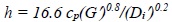 |
where cp is the specific heat of the gas at constant pressure, B.T.u./(lb.)(°F), G′ is the mass velocity, expressed as lb. of gas/sec./sq. ft, . . . and Di′ is in inches. Perry [10 Perry, J. H., 1950, Chemical Engineers’ Handbook, p. 467, McGraw-Hill.]
Note that the equation is dimensionally homogeneous because parameter symbols represent numerical value but not dimension, and the dimension units that underlie parameter symbols are specified in the accompanying nomenclature.
Equations in which parameter symbols represent numerical value but not dimension are still used, but not widely. Holman [11 Holman, J. O., 2009, Heat Transfer, 10th edition, Table 9-3, McGraw-Hill.] lists several dimensional equations including the following. The dimension units specified in the accompanying nomenclature are watts, meters, and Centigrade.
 |
10. THE TRANSFORMATION FROM q = hΔT TO ΔT = f{q} AND q = f{ΔT}
The transformation from q = hΔT to ΔT = f{q} and q = f{ΔT} requires that q and ΔT be separated in all equations that explicitly or implicitly include q/ΔT (ie include h).
Eq. (15)2 is an important equation in the analysis of heat transfer between two fluids separated by a flat wall. To separate q and ΔT, substitute q/ΔTtotal for U, q/ΔT1 for h1, q/ΔTwall for kwall/twall, and q/ΔT2 for h2, then separate q and ΔT, resulting in Eq. (16). Eqs. (15) and (16) are identical--they differ only in form. In the alternate view of homogeneity, Eq. (16) replaces Eq. (15).
 |
(15) |
 |
(16) |
Eq. (17) is a heat transfer coefficient correlation often used in the analysis of convective heat transfer. To separate q and ΔT, replace Nu with qD/ΔTk, then separate q and ΔT, resulting in Eq. (18). Note that, since Eq. (18) is not quantitative, it is not necessary to specify dimension units that underlie parameter symbols.
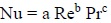 |
(17) |
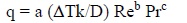 |
(18a) |
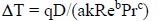 |
(18b) |
2 Text books often present Eq. (15) in the form U = 1/(1/h1 + twall/kwall+ 1/h2), a form that applies only if the relationship between q and ΔT1 and ΔT2 is proportional, and the wall is flat. Eq. (15) always applies if the wall is flat.
It is important to note that heat transfer coefficients cannot be measured directly. h values must be determined by measuring q and ΔT, then dividing q by ΔT. The separation of q and ΔT described above reverses the step in which q data are divided by ΔT data, and results in correlations in the desired form q = f{ΔT} or ΔT{q}.
11. THE SOLUTION OF PROPORTIONAL AND MODERATELY NONLINEAR HEAT TRANSFER PROBLEMS
Table 1 describes the solution of a moderately nonlinear heat transfer problem that concerns heat transfer between two fluids separated by a flat wall. The solution on the left side of Table 1 is based on q = hΔT. The solution on the right side is based on ΔT = f{q}. The solutions described in Table 1 are typical of problems in which the thermal behavior of boundary layers is described by equations (rather than charts).
Note the following in Table 1:
- The equations on the left side of Table 1 are identical to the equations on the right side. They differ only in form.
- The equation on the left side of Line 6 is much more difficult to solve because it contains three unknowns (U, ΔT1, and ΔT2), whereas the equation on the right side contains one unknown (q).
- The equation on the right side of Line 6 can be solved in about a minute using Excel and trial-and-error methodology. It would take much longer than a minute to solve the equation on the left side, and the likelihood of error would be much greater.
- If ΔT1 and ΔT2 were proportional to q--ie, if h1 and h2 were constants--the equations on both sides of Line 6, would be simple to solve. In other words, proportional problems are very simple to solve whether the solution is based on q = hΔT or ΔT = f{q}.
- The problem in Table 1 can be solved graphically if the solution is based on ΔT = f{q} because the equation on the right side of Line 1 can be solved graphically. The problem in Table 1 cannot be solved graphically if the solution is based on q = hΔT because the equation on the left side of Line 1 cannot be solved graphically.
12. THE SOLUTION OF A HIGHLY NONLINEAR HEAT TRANSFER PROBLEM
12.1. The Solution of a Highly Nonlinear Heat Transfer Problem Based on q = f{ΔT}
If ΔT2{q} in Table 1 were so highly nonlinear that it included a region in which dq/dΔT2 is negative, the relationship between q and ΔT2 would probably be described graphically in the form q vs ΔT2. The problem could have more than one solution, and operation might be thermally unstable in the region in which dq/dΔT2 is negative. Such problems are solved quite simply if the solution is based on q = f{ΔT}, as demonstrated by the following3:
- Use the given information to plot q vs (T2 + ΔT2{q}). Note that (T2 + ΔT2{q}) is the temperature of the interface that adjoins Fluid 2, and q is the heat flux out of that interface.
- On the same chart, use the given information to plot q vs (T1 - ΔT1 - ΔTwall). Note that (T1 - ΔT1 - ΔTwall) is the temperature of the interface that adjoins Fluid 2, and q is the heat flux into that interface.
- At intersections of the two curves, the heat flux into the interface in Fluid 2 equals the heat flux out of that interface. Therefore, intersections are steady-state operating points provided operation at the intersection is thermally stable.
- If an intersection is in a region in which dq/dΔT2 is negative, the operation may be thermally unstable. To appraise thermal stability at the intersection, inspect the chart to determine whether a small perturbation at the intersection would shrink or grow.
- If a small perturbation would shrink, operation at the intersection is thermally stable with respect to small perturbations. (It may be thermally unstable with respect to large perturbations.)
-
If a small perturbation would grow, operation at the intersection is thermally unstable.
- If the unstable intersection lies between two other intersections, inspection of the chart will indicate that the instability results in hysteresis.
- If there is only one intersection, inspection of the chart will indicate that the instability results in undamped oscillations in temperature and heat flux.
12.2. The Solution of Highly Nonlinear Heat Transfer Problems Based on q = hΔT
The solution of the highly nonlinear problem above is quite simple because the solution is based on q = f{ΔT}. If the solution is based on q = hΔT, the chart of q vs ΔT2 is replaced by a chart of h vs ΔT2 and the addition of the variable h adds so much complexity that it is virtually impossible to determine the correct and complete solution of the problem.
13. STRESS/STRAIN PROBLEMS
13.1. The Solution of Stress/Strain Problems in the Elastic Region Based on σ = Eelasticε and σ = f{ε}
In the elastic region:
- σ = Eelasticε is a proportional equation, and Eelastic is a dimensioned proportionality constant.
- σ = f{ε} is the proportional equation σ = cε, and c is a dimensionless proportionality constant.
- c is numerically equal to Eelastic.
Because both σ = Eelasticε and σ = cε are proportional equations, and because c and Eelastic are numerically equal, the solution of elastic problems based on σ = cε is identical to the solution based on σ = Eelasticε. The only difference between the two solutions is that the symbols in one equation represent numerical value and dimension, whereas the symbols in the other equation represent numerical value but not dimension.
13.2. Why Inelastic Stress/Strain Problems Are Much Simpler to Solve if the Solution is Based on σ = f{ε} Rather Than σ = Esecantε
In the inelastic region, E is the variable Esecant. Because σ = Esecantε contains three variables whereas σ = f{ε} contains two variables, inelastic problems are much simpler to solve if the solution is based on σ = f{ε}.
The bar problem below demonstrates that inelastic problems are much simpler to solve if the solutions are based on σ = f{ε} rather than σ = Esecantε.
13.3. The Solution of a Stress/Strain Problem Using σ = Eε.
Using modulus, determine the strain in the bar shown in the following sketch.
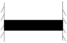
13.3.1. Given:
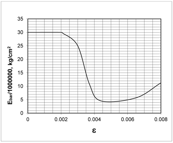
- The stress in the bar is 45,000 kg/cm2.
-
Ebar{ε} is described in Fig. (1
 ).
).
 |
Fig. (1) Bar modulus curve. |
13.4. Solve the Problem in Section 13.3 Using σ = f{ε}
Determine the strain in the bar.
13.4.1. Given:
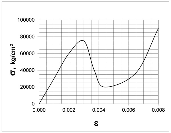
- The stress in the bar is 45,000 kg/cm2.
-
σ = f{ε} is described in Fig. (2
 ).
).
 |
Fig. (2) Bar stress/strain curve. |
13.4.2. Analysis and Solution
Inspection of Fig. (2) indicates that the strain in the bar may be .0015, .0036, or .0068. The given information is not sufficient to determine a unique solution.
13.4.3. The Purpose of the Bar Problem
The purpose of the bar problem is to demonstrate that it is much easier to solve inelastic problems if E is not used in the solution. If E is not used, the correct and complete solution of the bar problem requires less than ten seconds, and there is virtually no chance of error. If E is used, the correct and complete solution requires much longer than ten seconds, and there is a considerable chance of error because the problem does not have a unique solution.
14. WHY “STRESS/STRAIN CHARTS” ARE NOT CHARTS OF STRESS VS STRAIN, AND WHY “STRESS/STRAIN CHARTS” ARE IN PRECISELY THE FORM REQUIRED IN THE ALTERNATE VIEW OF HOMOGENEITY
It is important to note that charts never describe how parameters are related. They always describe how numerical values of parameters are related.
For example, stress/strain charts describe the equation σ = f{ε} in which σ and ε represent numerical value but not dimension. The dimension units that underlie σ and ε must be specified on the chart, or in an accompanying nomenclature. Note that if the dimension units were not specified on Figs. (1 and 2), the figures would not be quantitative.
In other words, charts are in precisely the form required in the alternate view of homogeneity because charts describe how numerical values are related.
CONCLUSION
The alternate view of dimensional homogeneity described herein should replace the current view, and engineering parameters and laws should be revised accordingly.
SYMBOLS
Note: Depending on the context in which a parameter symbol is used, parameter symbols may represent numerical value and dimension, or numerical value but not dimension,
| a | = acceleration |
| c | = proportionality constant |
| Cp | = heat capacity |
| D | = Diameter |
| E | = σ/ε |
| F | = Force |
| G | = mass velocity |
| h | = q/ΔT |
| I | = electric current |
| k | = q/(dT/dx) |
| Nu | = qD/(ΔTk) |
| Pr | = Cpμ/k |
| q | = heat flux |
| R | = V/I |
| Re | = DG/μ |
| s | = distance traveled |
| t | = thickness or elapsed time |
| T | = Temperature |
| Ti2 | = Temperature of the interface in Fluid 2 |
| U | = q/ΔTtotal |
| V | = average velocity or electromotive force in volts |
| ε | = strain |
| μ | = viscosity |
| σ | = stress |
CONSENT FOR PUBLICATION
Not applicable.
CONFLICT OF INTEREST
The authors declare no conflict of interest, financial or otherwise.
ACKNOWLEDGEMENTS
Declared none.
REFERENCES
| [1] | Galileo, 1638, Two New Sciences, P. 152, translation by Stillman Drake, published 1974 by The University of Wisconsin Press. |
| [2] | Newton, I., The Principia, 1726, 3rd edition, translation by Cohen, I. B. and Whitman, A. M., 1999, P. 460, University of California Press. |
| [3] | Fourier, J., 1822, The Analytical Theory of Heat, Article 160, 1955 Dover edition of the 1878 English translation, The University Press. |
| [4] | Langhaar, H. L., 1951, Dimensional Analysis and Theory of Models, P. 13, John Wiley & Sons. |
| [5] | Bird, Stewart, and Lightfoot, 1960, Transport Phenomena, P. 391, John Wiley and Sons, Inc. |
| [6] | Bejan, Adrian, 2013, Convection Heat Transfer, 4th edition, P. 32, John Wiley and Sons, Inc. [http://dx.doi.org/10.1002/9781118671627] |
| [7] | Adiutori, E. F., 1974, “The New Heat Transfer”, pp. 1-14, 1-15, Ventuno Press. |
| [8] | Adiutori, E. F., 1990, “Origins of the Heat Transfer Coefficient”, pp 46-50, Mechanical Engineering, August issue. |
| [9] | Maxwell, J. C., 1873, Electricity and Magnetism, pp. 295, 296, Macmillan. |
| [10] | Perry, J. H., 1950, Chemical Engineers’ Handbook, p. 467, McGraw-Hill. |
| [11] | Holman, J. O., 2009, Heat Transfer, 10th edition, Table 9-3, McGraw-Hill. |
Endorsements
Browse Contents
Table of Contents
- INTRODUCTION
- THE HISTORY OF DIMENSIONAL HOMOGENEITY
- THE MEANING OF ENGINEERING LAWS
- WHY PARAMETERS SUCH AS h, E, AND R ARE REQUIRED IF PARAMETER SYMBOLS REPRESENT NUMERICAL VALUE AND DIMENSION
- WHY PARAMETERS SUCH AS h, E, AND R CAN BE ABANDONED IF PARAMETER SYMBOLS REPRESENT NUMERICAL VALUE BUT NOT DIMENSION
- MAXWELL’S 1873 VIEW OF OHM’S LAW AND R
- ENGINEERING LAWS BASED ON THE ALTERNATE VIEW OF DIMENSIONAL HOMOGENEITY--ie BASED ON PARAMETER SYMBOLS THAT REPRESENT NUMERICAL VALUE BUT NOT DIMENSION
- COMPARING MATHEMATICAL ANALOGS OF ENGINEERING LAWS
- THE “DIMENSIONAL EQUATIONS” WIDELY USED IN MID-TWENTIETH CENTURY
- THE TRANSFORMATION FROM q = hΔT TO ΔT = f{q} AND q = f{ΔT}
- THE SOLUTION OF PROPORTIONAL AND MODERATELY NONLINEAR HEAT TRANSFER PROBLEMS
- THE SOLUTION OF A HIGHLY NONLINEAR HEAT TRANSFER PROBLEM
- STRESS/STRAIN PROBLEMS
- WHY “STRESS/STRAIN CHARTS” ARE NOT CHARTS OF STRESS VS STRAIN, AND WHY “STRESS/STRAIN CHARTS” ARE IN PRECISELY THE FORM REQUIRED IN THE ALTERNATE VIEW OF HOMOGENEITY
- CONCLUSION