- Home
- About Journals
-
Information for Authors/ReviewersEditorial Policies
Publication Fee
Publication Cycle - Process Flowchart
Online Manuscript Submission and Tracking System
Publishing Ethics and Rectitude
Authorship
Author Benefits
Reviewer Guidelines
Guest Editor Guidelines
Peer Review Workflow
Quick Track Option
Copyediting Services
Bentham Open Membership
Bentham Open Advisory Board
Archiving Policies
Fabricating and Stating False Information
Post Publication Discussions and Corrections
Editorial Management
Advertise With Us
Funding Agencies
Rate List
Kudos
General FAQs
Special Fee Waivers and Discounts
- Contact
- Help
- About Us
- Search


The Open Mechanical Engineering Journal
(Discontinued)
ISSN: 1874-155X ― Volume 14, 2020
Relation Between Convective Instability and Global Instability on a Rotating Disk
Lee Keunseob*, Nishio Yu, Izawa Seiichiro, Fukunishi Yu
Abstract
Background:
The velocity fluctuations grow dominantly by convective instability form 32 spiral vortices which are stationary with respect to the disk. However, recent researches suggest that the global instability plays a role in the boundary layer transition.
Objective:
The study looks into the relation between convective instability and global instability.
Method:
A finite difference method is used to carry out numerical simulation. The full Navier-Stokes perturbation equations and the continuity equation solved by simulation code.
Results:
A disturbance is continuatively introduced to excite the convectively unstable mode, which successfully generates a flow field with 32 spiral and stationary vortices. Next, a short-duration artificial disturbance with an azimuthal wavenumber of 64 is introduced at Reynolds number of 530 in order to introduce a velocity fluctuation of the traveling mode, which is globally unstable. It is shown that the source of vibration for the globally unstable mode exists between Reynolds number of 560 and 670. Finally, the global and traveling wavenumber 64 component is excited in a flow field which is dominated by the convective and stationary wavenumber 32 component. It is shown that the wavenumber 64 component grows by the global instability even when the excitation is very weak.
Conclusion:
The results suggest that the reason why the globally unstable mode has not been observed in experiments is because the boundary layer transition caused by the convective instability takes place before the globally unstable mode can start to grow by itself.
Article Information

Identifiers and Pagination:
Year: 2018Volume: 12
Issue: Suppl-1, M3
First Page: 37
Last Page: 53
Publisher Id: TOMEJ-12-37
DOI: 10.2174/1874155X01812010037
Article History:
Received Date: 30/05/2017Revision Received Date: 16/06/2017
Acceptance Date: 22/06/2017
Electronic publication date: 15/02/2018
Collection year: 2018
open-access license: This is an open access article distributed under the terms of the Creative Commons Attribution 4.0 International Public License (CC-BY 4.0), a copy of which is available at: (https://creativecommons.org/licenses/by/4.0/legalcode). This license permits unrestricted use, distribution, and reproduction in any medium, provided the original author and source are credited.
* Address correspondence to this author at the Department of Mechanical Systems Engineering, Tohoku University, Sendai, Miyagi, Japan, Tel: +81 22 7956929; Fax: +81 22 7956927; E-mail: keunseob@fluid.mech.tohoku.ac.jp
| Open Peer Review Details | |||
|---|---|---|---|
| Manuscript submitted on 30-05-2017 |
Original Manuscript | Relation Between Convective Instability and Global Instability on a Rotating Disk | |
1. INTRODUCTION
The boundary layer over a rotating disk becomes three-dimensional owing to the centrifugal force. The transition process of this boundary layer resembles that of a swept wing boundary layer which is also three-dimensional. And because the flow over a rotating disk is usually easier to handle compared to a swept wing flow, the boundary layer transition of a rotating disk flow has been enthusiastically studied in the past. There are three known groups of instabilities in a rotating disk flow, namely the convective, absolute and global instabilities. The convective instability is initiated by unavoidable minute roughness on a real disk continuatively supplying disturbance into the boundary layer. The amplitude of velocity fluctuation increases as they travel downstream. On the other hand, in the case of the absolute or global instabilities, once the flow is disturbed in their unstable region, the velocity fluctuation is self-sustained, and there is no need to continuatively supply a disturbance.
First, the convective instability was studied. In an experiment, Smith [1N. H. Smith, Exploratory investigation of laminar-boundary-layer oscillations on a rotating disk, .] detected sinusoidal waves in the transition region for the first time, using random disturbances to disturb the boundary layer. Gregory et al. [2N. Gregory, J.T. Stuart, and W.S. Walker, "On the stability of three-dimensional boundary layers with application to the flow due to a rotating disk", Philosophical Transactions of the Royal Society of London A: Mathematical, Physical and Engineering Sciences, vol. 248, no. 943, pp. 155-199.
[http://dx.doi.org/10.1098/rsta.1955.0013] ] clearly showed equi-angular spiral vortices around the Reynolds number of 430. Fedorov et al. [3B.I. Fedorov, G.Z. Plavnik, I.V. Prokhorov, and L.G. Zhukhovitskii, "Transitional flow conditions on a rotating disk", Journal of Engineering Physics and Thermophysics, vol. 31, no. 6, pp. 1448-1453.
[http://dx.doi.org/10.1007/BF00860579] ] observed the stationary and traveling mode vortices overlapped on the disk surface. Kobayashi et al. [4R. Kobayashi, Y. Kohama, and C. Takamadate, "Spiral vortices in boundary layer transition regime on a rotating disk", Acta Mech., vol. 35, no. 1, pp. 71-82.
[http://dx.doi.org/10.1007/BF01190058] ] and Kohama [5Y. Kohama, "Study on boundary layer transition of a rotating disk", Acta Mech., vol. 50, no. 3, pp. 193-199.
[http://dx.doi.org/10.1007/BF01170959] ] observed ring-like co-rotating vortices around each spiral vortex and attributed the transition to these small flow structures. An experimental study by Wilkinson & Malik [6S.P. Wilkinson, and M.R. Malik, "Stability experiments in the flow over a rotating disk", AIAA J., vol. 23, no. 4, pp. 588-595.
[http://dx.doi.org/10.2514/3.8955] ] showed that the spiral vortices came from discrete roughness disturbance on the disk. Corke & Knasiak [7T.C. Corke, and K.F. Knasiak, "Stationary travelling cross-flow mode interactions on a rotating disk", J. Fluid Mech., vol. 355, pp. 285-315.
[http://dx.doi.org/10.1017/S0022112097007738] ] conduced an experiment controlling the characteristics of the stationary modes using the artificial roughness on the disk, and showed that the traveling mode and stationary mode were overlapped in the nonlinear stage.
Theoretical studies of the convective instability have also been conducted. Kobayashi et al. [4R. Kobayashi, Y. Kohama, and C. Takamadate, "Spiral vortices in boundary layer transition regime on a rotating disk", Acta Mech., vol. 35, no. 1, pp. 71-82.
[http://dx.doi.org/10.1007/BF01190058] ] and Malik et al. [8M.R. Malik, S.P. Wilkinson, and S.A. Orszag, "Instability and transition in rotating disk flow", AIAA J., vol. 19, no. 9, pp. 1131-1138.
[http://dx.doi.org/10.2514/3.7849] ] conducted experimental and theoretical studies simultaneously and confirmed that a disturbance began to grow by the convective stationary cross-flow instability at Reynolds numbers of 261 and 287, respectively. They attributed the difference between the former theoretical results and experimental results for the critical Reynolds number to the effect of the Coriolis force and the streamline curvature, which are neglected in the linear stability theory. A theoretical study by Malik [9M.R. Malik, "The neutral curve for stationary disturbances in rotating-disk flow", J. Fluid Mech., vol. 164, pp. 275-287.
[http://dx.doi.org/10.1017/S0022112086002550] ] showed that the critical Reynolds numbers of the stationary mode for the inviscid type and viscous type were 285.36 and 440.88, respectively. Balakumar & Malik [10P. Balakumar, and M.R. Malik, "Traveling disturbances in rotating-disk flow", Theor. Comput. Fluid Dyn., vol. 2, no. 3, pp. 125-137.] also showed that the critical Reynolds numbers of the traveling mode for the inviscid type and the viscous type were 283.6 and 64.46, respectively. Hussain et al. [11Z. Hussain, S.J. Garrett, and S.O. Stephen, "The instability of the boundary layer over a disk rotating in an enforced axial flow", Phys. Fluids, vol. 23, no. 11, pp. 114-108.
[http://dx.doi.org/10.1063/1.3662133] ] indicated in their theoretical study that the streamline-curvature instability also had an important role in the axial flow, even though the flow was dominated by the cross-flow instability.
Lingwood [12R.J. Lingwood, "Absolute instability of the boundary layer on a rotating disk", J. Fluid Mech., vol. 299, pp. 17-33.
[http://dx.doi.org/10.1017/S0022112095003405] , 13R.J. Lingwood, "Absolute instability of the Ekman layer and related rotating flows", J. Fluid Mech., vol. 331, pp. 405-428.
[http://dx.doi.org/10.1017/S0022112096004144] ], in her theoretical study, pointed out the possibility of the absolute instability ruling the transition. The critical Reynolds number she estimated was 507, under an assumption of parallel flow. However, Itoh [14N. Itoh, "Structure of Absolute Instability in 3-D Boundary Layers: Part 1. Mathematical Formulation", Trans. Jpn. Soc. Aeronaut. Space Sci., vol. 44, no. 144, pp. 96-100.
[http://dx.doi.org/10.2322/tjsass.44.96] , 15N. Itoh, "Structure of absolute instability in 3-d boundary layers: Part 2. application to rotating-disk flow", Trans. Jpn. Soc. Aeronaut. Space Sci., vol. 44, no. 144, pp. 101-105.
[http://dx.doi.org/10.2322/tjsass.44.101] ] showed that under a slightly non-parallel-flow condition, the flow field became stable for absolute instability. Davies & Carpenter [16C. Davies, and P.W. Carpenter, "Global behaviour corresponding to the absolute instability of the rotating-disc boundary layer", J. Fluid Mech., vol. 486, pp. 287-329.
[http://dx.doi.org/10.1017/S0022112003004701] ] in their numerical simulation showed that, in a non-parallel flow field, the velocity fluctuation consequently grew by the convective instability. Moreover, Othman & Corke [17H. Othman, and T.C. Corke, "Experimental investigation of absolute instability of a rotating-disk boundary layer", J. Fluid Mech., vol. 565, pp. 63-94.
[http://dx.doi.org/10.1017/S0022112006001546] ] found that the amplitude of wave packets increased linearly even in the unstable region of the absolute instability, which was downstream of the critical Reynolds number of 507. These research results imply that global instability, which does not assume a parallel-flow condition, is more important than absolute instability.
Appelquist et al. [18E. Appelquist, P. Schlatter, P.H. Alfredsson, and R.J. Lingwood, "On the global nonlinear instability of the rotating-disk flow over a finite domain", J. Fluid Mech., vol. 803, pp. 332-355.
[http://dx.doi.org/10.1017/jfm.2016.506] ], in their study solving the full Navier-Stokes equations, suggested that the globally unstable mode started at the Reynolds number of 583. Although the past researches on the global instability focused in the region around Re = 507, which was the critical Reynolds number for the absolute instability, we believe more attention should be paid to the area around or downstream of Reynolds number 583.
In this study, we conducted a nonlinear numerical simulation to investigate the relation between convective instability and global instability. In experiments, it is almost impossible to avoid strong velocity fluctuations deriving from the convective instability dominating the flow field. So, a numerical simulation is the best choice for this kind of research. The remainder of this paper is organized as follows. Section 2 shows the numerical method and conditions. The relations between the convective instability and global instability are presented and discussed in section 3. Our conclusions are given in section 4.
2. NUMERICAL FORMULATION AND NUMERICAL PROCEDURES
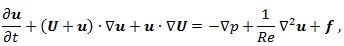
Numerical simulation is carried out using the finite difference method. The simulation code solves the full Navier-Stokes perturbation equations,
 |
(1) |
and the continuity equation,
 |
(2) |
where U = (U,V,W) are the radial, azimuthal and wall-normal components of the base-flow velocities, while u = (u,v,w) are those of the corresponding perturbation velocities in cylindrical polar coordinates. In the equation, is pressure, t is time, and f is the forcing term used in the sponge regions. The length
 , the rotational velocity r*Ω*, the pressure (r*Ω*)2p and the time scale
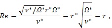
 are used to nondimensionalize all the variables in the above equations, where Ω* is the angular velocity, v is the kinematic viscosity, p is the density, and the superscript * denotes dimensional values. Therefore, the Reynolds number is defined as
 |
(3) |
indicating that this Reynolds number Re is identical to the nondimensionalized radial position r on the disk. Hereafter, the number of disk rotations, which is given by T = t*Ω*/2π, is employed to scale time.
The full Navier-Stokes perturbation equations and the continuity equations are calculated by the MAC method. The second-order Crank-Nicolson semi-implicit scheme is used for time advancement. The third-order upwind scheme (Kawamura-Kuwahara scheme [19T. Kawamura, H. Takami, and K. Kuwahara, "Computation of high Reynolds number flow around a circular cylinder with surface roughness", Fluid Dyn. Res., vol. 1, no. 2, pp. 145-162.
[http://dx.doi.org/10.1016/0169-5983(86)90014-6] ]) is applied in the convection terms, and the fourth-order central difference scheme is applied for the other terms. A 27-color SOR method is used to compute the Poisson equation, because our program is written in CUDA language to be used in a multi-GPU platform.
2.1. Computational Domain
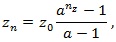
Fig. (1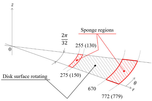 ) shows the computational domains, and Table (1). lists the computational parameters. For reducing the computational cost, the domain is limited to a fan-shaped region instead of a full circular disk. The narrower domain (255 ≤ r ≤ 772) and wider domain (130 ≤ r ≤ 779) computations with different sizes in the radial direction are carried out. In both cases the domain sizes in other directions are 0 ≤ θ ≤ 2π/32 and 0 ≤ z ≤ 54. For the azimuthal direction, periodic boundary conditions are used, and because the azimuthal size is 2π/32, fluctuations with an azimuthal wavenumber of 32 and its multiples appear in the flow field. For the wall-normal direction, the grids are distributed according to a starting wall-normal location of z 0 and a geometric series of a common ratio of a. The grid locations in the wall-normal direction are,
 |
(4) |
where the n-th grid in the wall-normal direction is nz. The values of a and z 0 are given in (Table 1).
 |
Fig. (1) Computational domain. |
2.2.. Initial Condition and Boundary Conditions
The von Kármán similarity solution is adopted for the base velocity components. As an initial condition, the perturbation velocities and pressure components are all set to zero. For the boundary conditions, the perturbation components are set as u = 0, v = 0 and dw/dz = p at the upper boundary, which are identical to the values in Appelquist et al. [18E. Appelquist, P. Schlatter, P.H. Alfredsson, and R.J. Lingwood, "On the global nonlinear instability of the rotating-disk flow over a finite domain", J. Fluid Mech., vol. 803, pp. 332-355.
[http://dx.doi.org/10.1017/jfm.2016.506] ]. The perturbation velocities are zero at the upstream and downstream boundaries, which are in the radial direction. The periodic boundary condition is applied in the azimuthal direction. The Neumann condition for the pressure is used at all boundaries except for the upper boundary. Sponge regions are used in order to prevent nonphysical reflections at the upstream and downstream boundaries. The sponge function is given by
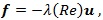 |
(5) |
where the λ(Re) is defined as
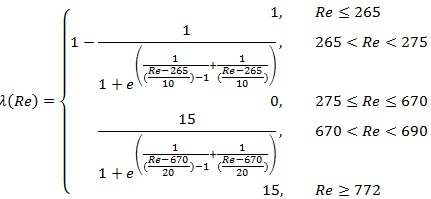 |
(6) |
 |
(7) |
Equations (6) and (7) indicate where the sponge functions are in the narrower domain case and the wider domain case, respectively. Therefore, the actual computational region is between the two sponge regions. In the sponge regions, the perturbation velocities are forced to decrease.
2.3. Artificial Disturbances
An artificial disturbance is added in the form of a wall-normal suction and blowing from the disk surface. The disturbance is defined as,
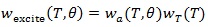 |
(8) |
where wa(T θ) is the azimuthal amplitude, and wT(T) is the temporal amplitude. wa(T θ) is given by
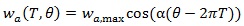 |
(9) |
Fig. (2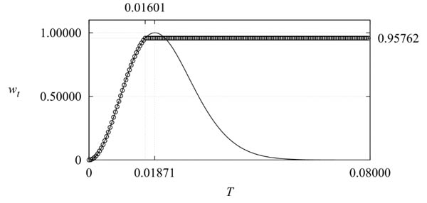 ) shows the temporal amplitude of the artificial disturbance. The amplitudes of the continuative disturbance to excite the convectively unstable mode at the beginning of the computation are shown by the circles in Fig. (2). At T = 0.01601, the amplitude reaches 0.95762, and after that, this amplitude is maintained.
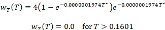 |
(10) |
 |
Fig. (2) The temporal amplitude of the artificial disturbance wT(T). |
In the wider domain case, the disturbance with the maximum amplitude wa,max of 10-5V is added at Re = 253 ~ 257. In the narrower domain case, the maximum amplitude wa,max is 10-11V, and is added at Re = 283 ~ 287. The wavenumber of disturbance α is 32 for both cases. The curved line in Fig. (2) is the amplitude of the disturbance to excite the globally
unstable mode. The excitation of the globally unstable mode is carried out only in the narrower domain. The temporal amplitude is given by,
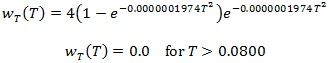 |
(11) |
At T = 0.01871, the temporal amplitude reaches its maximum. The maximum amplitudes wa,max are 10-6V, 10-8V and
10-10V. For the azimuthal amplitude wa,max 10-6V case, the disturbance is introduced at Re = 528 ~ 532. When the maximum amplitudes wa,max are 10-8V and 10-10V, the disturbances are introduced at Re = 588 ~ 592. In the excitation of global instability, the wavenumber of disturbance α is 64.
3. RESULTS AND DISCUSSION
3.1. Code Verification by Convectively Unstable Mode Computation
A computation is carried out on the flow field where velocity fluctuations deriving from a convective instability are expected to take place, and compared with the experimental results to verify our computer code.
Fig. (3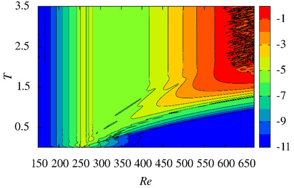 ) shows the spatio-temporal development of velocity fluctuations log(vrms) in the z = 1.3 plain. Strong wall-normal suction and blowing were carried out at the disk surface of Re ~ 255 in order to continuatively introduce a stationary disturbance with an azimuthal wavenumber of 32 into the flow field, which was expected to trigger convective instability downstream. The amplitude of the fluctuation of the wall-normal velocity was 10−5 of the azimuthal disk-surface velocity of the location. According to the theoretical study by Malik [9M.R. Malik, "The neutral curve for stationary disturbances in rotating-disk flow", J. Fluid Mech., vol. 164, pp. 275-287.
[http://dx.doi.org/10.1017/S0022112086002550] ], the critical Reynolds number for the stationary cross-flow convective type instability is 285.36. In experimental studies, 28 ~ 32 spiral vortices are observed [20S. Imayama, P.H. Alfredsson, and R.J. Lingwood, "A new way to describe the transition characteristics of a rotating-disk boundary-layer flow", Phys. Fluids, vol. 24, no. 3, p. 031701.
[http://dx.doi.org/10.1063/1.3696020] , 21S. Imayama, P.H. Alfredsson, and R.J. Lingwood, "Experimental study of rotating-disk boundary-layer flow with surface roughness", J. Fluid Mech., vol. 786, pp. 5-28.
[http://dx.doi.org/10.1017/jfm.2015.634] ]. In experiments, because of minute roughness on the disk surfaces, stationary disturbances are always supplied. After T = 2.0 in Fig. (3), the contour lines become vertical, which means the fluctuations have stopped growing and the flow field is in a steady state.
 |
Fig. (3) Spatio-temporal development of log(vrms) in the z = 1.3 plane. A strong artificial disturbance with azimuthal wavenumber of 32 is continuatively supplied at Re ~ 255. |
Fig. (4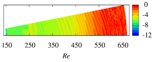 ) shows the color map of log|v| in z = 1.3 plane at T = 3.5 under the same condition. A finger-like pattern is clearly visible. It should be noted that two finger-like patterns correspond to one spiral vortex because the absolute value of the azimuthal velocity fluctuation is shown in the figure. So, there is only one spiral vortex in the flow field shown in the figure. The number of the spiral vortices will be 32 for the entire disk. The stripe pattern starts at Re = 255, and its strength increases in the radial direction. After Re > 600, a turbulent region can be observed. The location is not far from the locations observed in experiments.
 |
Fig. (4) Color map of log|v| in the z = 1.3 plane at T = 3.5 when the strong disturbance is continuatively introduced at Re ~ 255. |
Fig. (5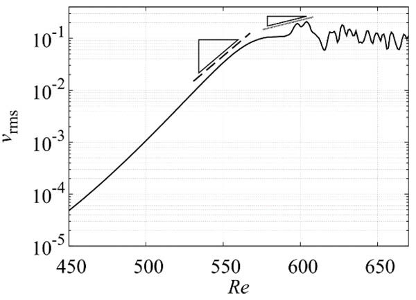 ) shows the RMS value of vrms of the same condition in the z = 1.3 plane at T = 3.5. The distribution of the RMS values shows that until Re ~ 560, the disturbance grows exponentially. This trend is close to the experimental results by Imayama et al. [20S. Imayama, P.H. Alfredsson, and R.J. Lingwood, "A new way to describe the transition characteristics of a rotating-disk boundary-layer flow", Phys. Fluids, vol. 24, no. 3, p. 031701.
[http://dx.doi.org/10.1063/1.3696020] ], in which 32 spiral vortices appeared “naturally” without any artificial disturbances except for the minute imperfectness of the disk surface. The wall-normal distribution of the RMS values of azimuthal velocity fluctuations at Re = 510 is shown in Fig. (6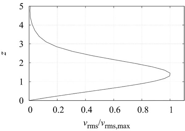 ). The distribution matches very well with the experimental data of Imayama et al. [21S. Imayama, P.H. Alfredsson, and R.J. Lingwood, "Experimental study of rotating-disk boundary-layer flow with surface roughness", J. Fluid Mech., vol. 786, pp. 5-28.
[http://dx.doi.org/10.1017/jfm.2015.634] ].
 |
Fig. (5) RMS values of vrms in the z = 1.3 plane at T = 3.5 when the strong disturbance is continuatively introduced at Re ~ 255. The solid line is our simulation result. The exponential fitting lines from experimental result (Imayama et al. [20S. Imayama, P.H. Alfredsson, and R.J. Lingwood, "A new way to describe the transition characteristics of a rotating-disk boundary-layer flow", Phys. Fluids, vol. 24, no. 3, p. 031701. [http://dx.doi.org/10.1063/1.3696020] ]) are given as vrms ~ exp(αRe), where α is the growth rate. For the dashed line and the dotted line, the values of α are 0.058 and 0.017. |
 |
Fig. (6) The RMS value of the azimuthal velocity fluctuation at Re = 510 when the strong disturbance is continuatively introduced at Re ~ 255. The profile is normalized by the maximum value. |
Fig. (7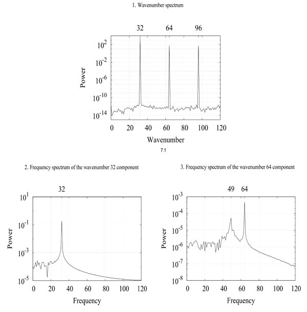 ) shows the spatial power spectra and the temporal power spectra of the azimuthal velocity at z = 1.3 and Re = 510. In Fig. (7.1), the data for the entire disk, which were constructed by copying the data of the 2π/32 domain at T = 3.5, were used to calculate the spatial power spectra. The dominant wavenumber is 32 and its harmonics components are present. This result is the reflection of 32 spiral vortices governing the flow field. Next, 250 temporal data points that cover T = 2.5 ~ 3.5 were used to calculate the temporal power spectra, which are shown in Figs. (7.2 and 7.3). The frequency resolution in these figures is 1. The frequency indicates the wavenumber per one rotation of the disk. The finding that the wavenumber and the frequency are both 32 indicates that the 32 spiral vortices are stationary with respect to the disk surface, which is consistent with the previously reported experimental results. Both in our computation, in which the flow field was excited by artificial disturbance at an upstream location of Re ~ 255, and the experimental data of Imayama et al. [20S. Imayama, P.H. Alfredsson, and R.J. Lingwood, "A new way to describe the transition characteristics of a rotating-disk boundary-layer flow", Phys. Fluids, vol. 24, no. 3, p. 031701.
[http://dx.doi.org/10.1063/1.3696020] , 21S. Imayama, P.H. Alfredsson, and R.J. Lingwood, "Experimental study of rotating-disk boundary-layer flow with surface roughness", J. Fluid Mech., vol. 786, pp. 5-28.
[http://dx.doi.org/10.1017/jfm.2015.634] ], in which the disturbance was only naturally provided from the disk surface, the velocity fluctuations were stationary with respect to the disk surfaces and their wavenumbers or the number of spiral vortices were similar. It can be judged that the velocity fluctuation in this computation grew by the convective instability as in experiments.

By carefully examining Fig. (7.3), it can be seen that the wavenumber 64 component has the frequencies of 49 and 64. The frequency of 64 is just the harmonic of the 32 component, but the frequency of 49 is not. This result suggests that a pattern of 64 spiral vortices that is traveling at a slower angular velocity than the disk surface co-exists in the flow field.
A computation to verify our simulation code was carried out and the results were compared to the existing experimental results. It was found that our simulation code could successfully calculate the flow field, which was governed by the stationary mode of convective instability, and the results were in good agreement with the experimental results.
3.2. Computation for the Convectively Unstable Mode with a much Weaker Stimulation
An additional simulation concerning the stationary convective instability was carried out using a much weaker artificial disturbance to excite the flow. The amplitude of the fluctuation of the wall-normal velocity was reduced from 10−5 to 10−11 of the azimuthal disk-surface velocity of the location. The reason for this reduction was to delay the growth of the velocity fluctuations related to stationary and convective instability, which was necessary in order to investigate the relation of this growth with the velocity fluctuations derived from global instability, which will be carried out later in this paper.
Fig. (8 ) shows the spatio-temporal development of the RMS value log(vrms) in the z = 1.3 plane when the weaker artificial disturbance was continuatively introduced at Re ~ 285. Fig. (8.1), which shows the unfiltered data, corresponds to Fig. (3) in the stronger disturbance case. A similar trend is observed between the cases with weaker and stronger disturbance, but the turbulent region does not appear downstream in the weaker disturbance case. The filtered data showing only the wavenumber 32 component is presented in Fig. (8.2). The figure is very close to Fig. (8.1). The RMS values of the wavenumber 64 component are shown in Fig. (8.3). The higher harmonics components are much smaller compared to the wavenumber 32 components.
 |
Fig. (8) Spatio-temporal development of log(vrms) in the z = 1.3 plane. The weaker artificial disturbance is continuatively introduced at Re ~ 285. |
Fig. (9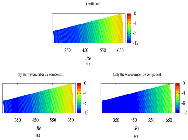 ) shows the color map of log|v| in the z = 1.3 plane at T = 3.0, which is the flow pattern, when the weaker disturbance is introduced at Re ~ 285. In Figs. (9.1 and 9.2), patterns corresponding to 32 spiral vortices can be observed. In Fig. (9.3), spiral patterns corresponding to a wavenumber of 64 can be found, but they are weaker than the wavenumber 32 component.
 |
Fig. (9) Color maps of log|v| in the z = 1.3 plane at T = 3.0 when the weaker disturbance is continuatively introduced at Re ~ 285. |
Fig. (10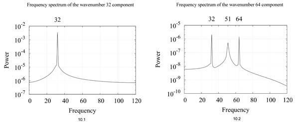 ) shows the temporal power spectra of the azimuthal velocity measured at z = 1.3 and Re = 630, when the weaker disturbance is added at Re ~ 285. The data are from T = 2.0 ~ 3.0. For the wavenumber 32 component, the peak frequency is at 32, showing that the spiral vortices of wavenumber 32 are stationary with respect to the disk surface. For the wavenumber 64 component, the frequency peaks are at 32, 51 and 64. It should be noted that the frequency peak of 51 is a traveling mode and not stationary. The frequency of 51 is very close to that of 49 found in Fig. (7.3), when the stronger disturbance was used.
3.3. Computation for the Globally Unstable Mode
In order to study the global instability, two computations having different locations for the start of the downstream sponge regions, namely Re = 560 and 670, were conducted. The other simulation conditions were the same for both cases. Fig. (11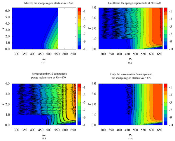 ) shows the spatio-temporal development of the RMS value of azimuthal velocity fluctuations log(vrms) in the z = 1.3 plane. Fig. (11) shows the RMS value for unfiltered azimuthal velocity fluctuations when the sponge region started at Re = 560. Figs. (11.1, 11.2 and 11.3) shows the RMS values for the cases with unfiltered data, the wavenumber 32 component filtered out and the wavenumber 64 component filtered out, respectively, when the sponge region started at Re = 630. In all cases, the short-duration artificial disturbance for the wavenumber 64 component was introduced at Re ~ 530. When the downstream sponge region started at Re = 560, the artificial disturbance is convected downstream, and disappears from this flow field after T = 6.5. On the other hand, when the downstream sponge region started at Re = 670, initially, the artificial disturbance is convected downstream, but after T = 1.0, the velocity fluctuation distribution stops changing. It is the global instability which allows the velocity fluctuation to sustain itself. This result suggests that the source of vibration for the globally unstable mode exists somewhere between Re = 560 and 670. In Fig. (11.2), the contour lines strongly oscillate upstream. This noisy region derives from the wavenumber 32 component as can be found in Fig. (11.3). Comparing Figs. 11.2 and 11.4), it is clear that the wavenumber 64 component is dominant in this case. Figs. (12.1, 12.2 and 12.3
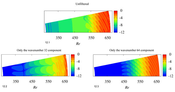 ) shows the color map of log|v| in the z = 1.3 plane at T = 4.0. This figure also confirms that the wavenumber 64 component is dominant.
 |
Fig. (10) Frequency spectra of v at z = 1.3 and Re = 630, for T = 2.0 ~ 3.0, when the weaker disturbance is continuatively introduced at Re ~ 285. |
 |
Fig. (11) Spatio-temporal development of log(vrms) in the z = 1.3 plane for the globally stable and unstable cases. The short-duration artificial disturbance is introduced at Re ~ 530. |
 |
Fig. (12) Color maps of log |v| in the z = 1.3 plane at T = 4.0 when a short-duration disturbance is introduced at Re ~ 530. |
Fig. (13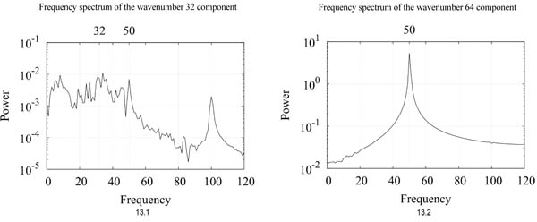 ) shows the temporal power spectra of the azimuthal velocity at z = 1.3 and Re = 630, using data of T = 3.0 ~ 4.0. The peak frequency of 50 is obviously the dominant frequency in the wavenumber 64 component shown in Fig. (13.2). The same frequency of 50 also appears in the wavenumber 32 component spectrum in Fig. (13.1). This peak corresponds to a traveling mode structure that is moving slower than the rotating disk. It should be noted that the frequency measured for the present structure of the traveling mode, namely 50, is very close to the frequencies measured for the two traveling mode structures which were found in the convective instability-dominated flow cases, namely 49 and 51, that were presented above. This result indicates that all these traveling mode structures were grown by the global instability.
 |
Fig. (13) Frequency spectra of v at z = 1.3 and Re = 630, for T = 3.0 ~ 4.0. A short-duration disturbance is introduced at Re ~ 530. |
Fig. (14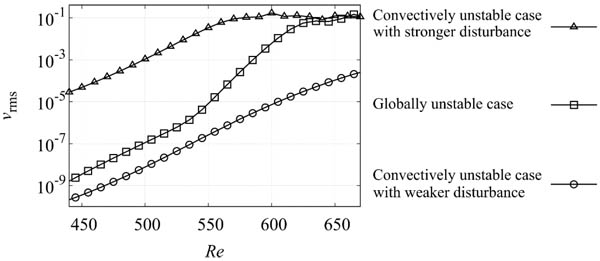 ) shows the RMS values of vrms at z = 1.3 for the last rotation. The growth rates of the RMS values for the convectively unstable flow fields and the globally unstable flow field are similar upstream of Re < 540. However, a difference in the growth rates of the RMS values between the convectively unstable flow fields and the globally unstable flow field is observed downstream of Re > 550. Interestingly, in the convectively unstable flow field in which

the weaker continuative disturbance is introduced upstream, the traveling mode for the 64 component, which can be grown by the global instability, could not grow as much as that in the globally unstable flow field.
3.4. Computation for the Relation between the Convectively Unstable Mode and Globally Unstable Mode
At Re ~ 590, where the source of the vibration for the global instability exists, the short-duration artificial disturbance for the wavenumber 64 component was introduced into the convectively unstable flow field when the weaker continuative disturbance was introduced upstream. Two amplitudes cases for the short-duration artificial disturbance were tried: a case with weaker disturbance and a case with stronger disturbance. The weaker disturbance had vrms~ 10−10, which was lower than the vrms of ~ 10−6 in the convectively unstable flow field at Re = 590. The stronger disturbance had vrms ~ 10−4, which was stronger than the vrms of ~ 10−6 in the convectively unstable flow field at Re = 590.
Fig. (15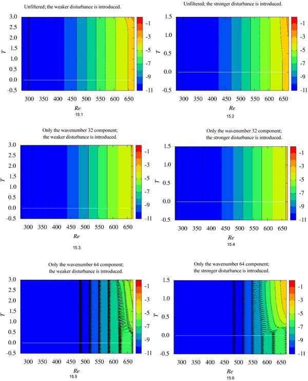 ) shows the spatio-temporal development of the RMS value log(vrms) at z = 1.3 for two disturbance cases mentioned above. For T = -0.5 ~ 0.0, the flow field is identical with the convectively unstable flow field for T = 2.5 ~ 3.0 when the weaker continuative disturbance was introduced upstream. Figs. (15.1, 15.3 and 15.5) shows the short-duration weaker disturbance case. Figs. (15.2, 15.4 and 15.6) shows the short-duration stronger disturbance case. In Figs. (15.1 and 15.2), which shows the unfiltered flow field, the short-duration disturbance is grown by the global instability. The diagrams for the 64 component (Figs. 15.5 and 15.6) clearly show that the global instability is excited. The diagrams for the 32 component (Figs. 15.3 and 15.4) show that the convective instability is continuously sustained. Interestingly, in the case of the short-duration weaker disturbance, although the artificial disturbance was much smaller than the convectively unstable flow field, which was stationary, the traveling global instability mode could be excited.
Fig. (16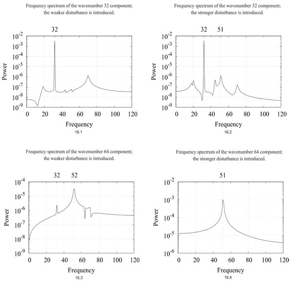 ) shows the temporal power spectra of the azimuthal velocity at z = 1.3 and Re = 630, for the last rotation in both types of disturbance. In Figs. 16.1 and 16.3), the short-duration weaker disturbance was introduced at Re = 590. In Figs. (16.2 and 16.4), the short-duration strong disturbance was introduced at Re = 590. In both disturbance cases, the wavenumber 32 component is the same, with a frequency of 32, and the wavenumber 64 component has frequencies of 52 or 50, which are similar to the frequency of 50 in the globally unstable flow field. Therefore, the 32 component was grown as a stationary mode by the convective instability and the 64 component was grown as a the traveling mode by the global instability, in both disturbance cases.
CONCLUSION
The relations between the velocity fluctuations deriving from the convective instability and from the global instability were studied using direct numerical simulations. In this study, we investigated cases in which the flow was disturbed in three different ways-namely, by the convectively unstable mode, by the globally unstable mode, and by both modes.

 |
Fig. (16) Frequency spectra of v at z = 1.3 and Re = 630, using the data of the last rotation. |
First, in order to excite the convectively unstable mode velocity fluctuation, wall-normal suction and blowing with an azimuthal wavenumber of 32 were continuously introduced at Re ~ 255. The amplitude of the wall-normal velocity component of the disturbance was 10-5V. After the flow reached a steady state, 32 spiral vortices were clearly observed upstream of Re=600, followed by a turbulent region downstream. The 32 spiral vortices were stationary, moving with the disk surface. This feature agreed with many of the previously reported experiments. The flow field did not change substantially even when the amplitude of the wall-normal velocity component of the introduced disturbance was reduced to 10-11V, and the location to introduce disturbance was changed to Re = 285.
Computations exciting the global unstable mode were carried out for two cases. Only the locations where the downstream sponge regions started were different, namely Re = 560 and 670. In both cases, the short-duration artificial disturbance with a wavenumber of 64 was introduced at Re ~ 530 only at the start of the computation. When the downstream sponge region started from Re = 560, the disturbance flowed downstream and the flow field returned to the perfectly laminar flow after 6.5 disk-rotations. However, when the downstream sponge region started from Re = 670, the disturbance was first convected downstream, but after one disk-rotation, the disturbed flow field began to sustain itself by the global instability. This result suggested that the source of vibration for the globally unstable mode existed somewhere between Re = 560 and 670. In the flow field, the 64 spiral vortices were dominant, and moved slower than the disk rotation-i.e., they were in the “traveling mode.” All the traveling mode structures were moving with a similar relative velocity against the disk surface, which suggested that all of them were grown by the global instability.
The flow field where interactions between the convectively unstable mode and the globally unstable mode took place was investigated. The disturbance with the wavenumber of 32 was constantly introduced into Re = 285 in order to excite the convectively unstable mode. After the flow field reached a steady state, the flow field was disturbed in a different manner, using a short-duration disturbance with a wavenumber of 64 at the downstream location of Re = 590. Two cases with different amplitudes of the second disturbance were tested. There was a 100-fold difference in the amplitudes of the disturbances between the two cases. In both cases, the wavenumber 64 component was successfully excited, and started to grow soon after the short-duration disturbance was introduced. It was interesting that the wavenumber 64 component which was excited later could grow even though the amplitude of the short-duration disturbance was much smaller than the amplitude of the wavenumber 32 component at the location, and also the wavenumber 32 component was of the stationary mode. It was also observed that the traveling wavenumber 64 component did not appear to affect the stationary wavenumber 32 component.
The results suggest that the reason why the globally unstable mode is not observed in experiments is because laminar-turbulent transition caused by the convective instability takes place before the flow reaches the Reynolds number where the global unstable mode can grow in a self-sustaining manner. Therefore, if there were a way to make the disk surface much cleaner in the experiments, we would be able to observe the growth of the traveling globally unstable mode.
LIST OF ABBREVIATIONS
| u | = perturbation velocities |
| U | = Base-flow velocities |
| t | = time |
| p | = Pressure |
| f | = Forcing term for the sponge regions |
| ν | = Kinematic viscosity |
| Ω | = Angular velocity |
| T | = The number of disk rotations |
| Re | = Reynolds number |
| ε | = Angle of a spiral vortex |
| α | = Wavenumber of disturbance |
| β | = Azimuthal division number |
CONSENT FOR PUBLICATION
Not applicable.
CONFLICT OF INTEREST
The authors declare no conflict of interest, financial or otherwise.
ACKNOWLEDGEMENTS
Declared none.
REFERENCES
| [1] | N. H. Smith, Exploratory investigation of laminar-boundary-layer oscillations on a rotating disk, . |
| [2] | N. Gregory, J.T. Stuart, and W.S. Walker, "On the stability of three-dimensional boundary layers with application to the flow due to a rotating disk", Philosophical Transactions of the Royal Society of London A: Mathematical, Physical and Engineering Sciences, vol. 248, no. 943, pp. 155-199. [http://dx.doi.org/10.1098/rsta.1955.0013] |
| [3] | B.I. Fedorov, G.Z. Plavnik, I.V. Prokhorov, and L.G. Zhukhovitskii, "Transitional flow conditions on a rotating disk", Journal of Engineering Physics and Thermophysics, vol. 31, no. 6, pp. 1448-1453. [http://dx.doi.org/10.1007/BF00860579] |
| [4] | R. Kobayashi, Y. Kohama, and C. Takamadate, "Spiral vortices in boundary layer transition regime on a rotating disk", Acta Mech., vol. 35, no. 1, pp. 71-82. [http://dx.doi.org/10.1007/BF01190058] |
| [5] | Y. Kohama, "Study on boundary layer transition of a rotating disk", Acta Mech., vol. 50, no. 3, pp. 193-199. [http://dx.doi.org/10.1007/BF01170959] |
| [6] | S.P. Wilkinson, and M.R. Malik, "Stability experiments in the flow over a rotating disk", AIAA J., vol. 23, no. 4, pp. 588-595. [http://dx.doi.org/10.2514/3.8955] |
| [7] | T.C. Corke, and K.F. Knasiak, "Stationary travelling cross-flow mode interactions on a rotating disk", J. Fluid Mech., vol. 355, pp. 285-315. [http://dx.doi.org/10.1017/S0022112097007738] |
| [8] | M.R. Malik, S.P. Wilkinson, and S.A. Orszag, "Instability and transition in rotating disk flow", AIAA J., vol. 19, no. 9, pp. 1131-1138. [http://dx.doi.org/10.2514/3.7849] |
| [9] | M.R. Malik, "The neutral curve for stationary disturbances in rotating-disk flow", J. Fluid Mech., vol. 164, pp. 275-287. [http://dx.doi.org/10.1017/S0022112086002550] |
| [10] | P. Balakumar, and M.R. Malik, "Traveling disturbances in rotating-disk flow", Theor. Comput. Fluid Dyn., vol. 2, no. 3, pp. 125-137. |
| [11] | Z. Hussain, S.J. Garrett, and S.O. Stephen, "The instability of the boundary layer over a disk rotating in an enforced axial flow", Phys. Fluids, vol. 23, no. 11, pp. 114-108. [http://dx.doi.org/10.1063/1.3662133] |
| [12] | R.J. Lingwood, "Absolute instability of the boundary layer on a rotating disk", J. Fluid Mech., vol. 299, pp. 17-33. [http://dx.doi.org/10.1017/S0022112095003405] |
| [13] | R.J. Lingwood, "Absolute instability of the Ekman layer and related rotating flows", J. Fluid Mech., vol. 331, pp. 405-428. [http://dx.doi.org/10.1017/S0022112096004144] |
| [14] | N. Itoh, "Structure of Absolute Instability in 3-D Boundary Layers: Part 1. Mathematical Formulation", Trans. Jpn. Soc. Aeronaut. Space Sci., vol. 44, no. 144, pp. 96-100. [http://dx.doi.org/10.2322/tjsass.44.96] |
| [15] | N. Itoh, "Structure of absolute instability in 3-d boundary layers: Part 2. application to rotating-disk flow", Trans. Jpn. Soc. Aeronaut. Space Sci., vol. 44, no. 144, pp. 101-105. [http://dx.doi.org/10.2322/tjsass.44.101] |
| [16] | C. Davies, and P.W. Carpenter, "Global behaviour corresponding to the absolute instability of the rotating-disc boundary layer", J. Fluid Mech., vol. 486, pp. 287-329. [http://dx.doi.org/10.1017/S0022112003004701] |
| [17] | H. Othman, and T.C. Corke, "Experimental investigation of absolute instability of a rotating-disk boundary layer", J. Fluid Mech., vol. 565, pp. 63-94. [http://dx.doi.org/10.1017/S0022112006001546] |
| [18] | E. Appelquist, P. Schlatter, P.H. Alfredsson, and R.J. Lingwood, "On the global nonlinear instability of the rotating-disk flow over a finite domain", J. Fluid Mech., vol. 803, pp. 332-355. [http://dx.doi.org/10.1017/jfm.2016.506] |
| [19] | T. Kawamura, H. Takami, and K. Kuwahara, "Computation of high Reynolds number flow around a circular cylinder with surface roughness", Fluid Dyn. Res., vol. 1, no. 2, pp. 145-162. [http://dx.doi.org/10.1016/0169-5983(86)90014-6] |
| [20] | S. Imayama, P.H. Alfredsson, and R.J. Lingwood, "A new way to describe the transition characteristics of a rotating-disk boundary-layer flow", Phys. Fluids, vol. 24, no. 3, p. 031701. [http://dx.doi.org/10.1063/1.3696020] |
| [21] | S. Imayama, P.H. Alfredsson, and R.J. Lingwood, "Experimental study of rotating-disk boundary-layer flow with surface roughness", J. Fluid Mech., vol. 786, pp. 5-28. [http://dx.doi.org/10.1017/jfm.2015.634] |