- Home
- About Journals
-
Information for Authors/ReviewersEditorial Policies
Publication Fee
Publication Cycle - Process Flowchart
Online Manuscript Submission and Tracking System
Publishing Ethics and Rectitude
Authorship
Author Benefits
Reviewer Guidelines
Guest Editor Guidelines
Peer Review Workflow
Quick Track Option
Copyediting Services
Bentham Open Membership
Bentham Open Advisory Board
Archiving Policies
Fabricating and Stating False Information
Post Publication Discussions and Corrections
Editorial Management
Advertise With Us
Funding Agencies
Rate List
Kudos
General FAQs
Special Fee Waivers and Discounts
- Contact
- Help
- About Us
- Search


The Open Ornithology Journal
(Discontinued)
ISSN: 1874-4532 ― Volume 13, 2020
Seabirds At-Sea Surveys: The Line-Transect Method Outperforms the Point-Transect Alternative
François Bolduc1, *, David A. Fifield2
Abstract
Introduction:
Knowledge of seasonal distribution and abundance of species is paramount in identifying key areas. Field data collection and analysis must provide best information concerning seabirds at-sea to optimize conservation efforts.
Methods:
We tested whether modeling of detection probabilities, and density estimates with their coefficients of variation obtained from the point-transect method provided more robust and precise results than the more commonly used line-transect method. We subdivided our data by species groups (alcids, and aerialist species), and into two behavior categories (flying vs. swimming). We also computed density estimates from the strip-transect and point count methods, to relate differences between transect methods to their counterparts that do not consider a decreasing probability of detection with distance from the observer. We used data collected in the Gulf of St. Lawrence between 2009 and 2010 when observers simultaneously conducted line- and point-transect sampling.
Results:
Models of detection probability using the line-transect method had a good fit to the observed data, whereas detection probability histograms of point-transect analyses suggested substantial evasive movements within the 0-50 m interval. This resulted in point-transect detection probability models displaying poor goodness of fit. Line transects yielded density estimates 1.2-2.6 times higher than those obtained using the point-transect method. Differences in percent coefficients of variation between line-transect and point-transect density estimates ranged between 0.2 and 5.9.
Conclusion:
Using 300 m wide line-transects provided the best results, while other methods could lead to biased conclusions regarding species density in the local landscape and the relative composition of seabird communities among species and behavior groups.
Article Information

Identifiers and Pagination:
Year: 2017Volume: 10
First Page: 42
Last Page: 52
Publisher Id: TOOENIJ-10-42
DOI: 10.2174/1874453201710010042
Article History:
Received Date: 21/12/2016Revision Received Date: 01/03/2017
Acceptance Date: 21/03/2017
Electronic publication date: 16/05/2017
Collection year: 2017
open-access license: This is an open access article distributed under the terms of the Creative Commons Attribution 4.0 International Public License (CC-BY 4.0), a copy of which is available at: (https://creativecommons.org/licenses/by/4.0/legalcode). This license permits unrestricted use, distribution, and reproduction in any medium, provided the original author and source are credited.
* Address correspondence to this author at the Canadian Wildlife Service, Environment and Climate Change Canada, 801-1550 avenue d’Estimauville, Québec, QC, G1J 0C3, Canada; Tel: 418-640-2910; E-mail: francois.bolduc@canada.ca
| Open Peer Review Details | |||
|---|---|---|---|
| Manuscript submitted on 21-12-2016 |
Original Manuscript | Seabirds At-Sea Surveys: The Line-Transect Method Outperforms the Point-Transect Alternative | |
INTRODUCTION
Bird conservation planning often includes population objectives at various spatial scales, e.g., [1North American Waterfowl Management Plan. In: Plan Committee North American Waterfowl Management Plan 2004 Strategic Guidance: Strengthening the Biological Foundation Canadian Wildlife Service, US Fish and Wildlife Service, Secretaria de Medio Ambiente y Recursos Naturales 2004. ], and incorporates the maintenance or restoration of species distributions. Knowledge of the abundance and distribution of species across seasons is paramount in biodiversity conservation, but also in identifying key areas and potential threats. Seabird populations can be impacted by increasing marine oil and gas exploitation, shipping traffic, and offshore wind power generation worldwide [2Vosta M. Global changes and new trends within the territorial structure of the oil, gas and coal industries. Acta Oeconomic Pragen 2009; 2009(1): 45-59.
[http://dx.doi.org/10.18267/j.aop.3] -4Musial W, Ram B. Large-scale offshore wind power in the United States: Assessment of opportunities and barriers National Renewable Energy Laboratory. Colorado, US: Department of Energy 2010.]. Accordingly, efforts to acquire knowledge of seabird abundance and distribution are also increasing [5Grecian WJ, Witt MJ, Attrill MJ, et al. A novel projection technique to identify important at-sea areas for seabird conservation: An example using the Northern gannets breeding in the North East Atlantic. Biol Conserv 2012; 156: 43-52.
[http://dx.doi.org/10.1016/j.biocon.2011.12.010] , 6Montevecchi WA, Hedd A, McFarlane Tranquilla L, et al. Tracking seabirds to identify ecologically important and high risk marine areas in the western North Atlantic. Biol Conserv 2012; 156: 62-71.
[http://dx.doi.org/10.1016/j.biocon.2011.12.001] ].
Data on seabirds at-sea are often gathered via ship-based observers. Many protocols evolved from the work of Tasker et al. [7Tasker ML, Jones PH, Dixon T, Blake F. Counting seabirds at sea from ships: A review of methods employed and a suggestion for a standardized approach. Auk 1984; 101: 567-77.], where observers used the strip-transect technique to estimate seabird densities. Using this technique, detected birds are simply declared in or out transect. When practical, survey protocols often employ line-transect techniques where the observer uses predetermined distance intervals to measures the perpendicular distance from the observer to the birds to correct apparent densities for decreasing detection with distance [8Komdeur J, Bertelsen J, Cracknell G. Manual for aeroplan and ship surveys of waterfowl and seabirds, Slimbridge: IWRB Special Publication 1992.-11Gjerdrum C, Fifield DA, Wilhelm S. Eastern Canada seabirds at-sea (ECSAS) standardized protocol for pelagic seabird surveys from moving and stationary platforms, Technical Report Series. Canad Wildlife Serv 2012.].
Estimating densities of flying birds is especially problematic since they move at speeds far in excess of the survey platform, which can result in over-estimation of density [7Tasker ML, Jones PH, Dixon T, Blake F. Counting seabirds at sea from ships: A review of methods employed and a suggestion for a standardized approach. Auk 1984; 101: 567-77., 12Spear LB, Nur N, Ainley DG. Estimating absolute densities of flying seabirds using analyses of relative movements. Auk 1992; 109: 385-9.
[http://dx.doi.org/10.2307/4088211] ]. Solutions to this problem include use of the vector method [12Spear LB, Nur N, Ainley DG. Estimating absolute densities of flying seabirds using analyses of relative movements. Auk 1992; 109: 385-9.
[http://dx.doi.org/10.2307/4088211] ], or the implementation of snapshot counts [7Tasker ML, Jones PH, Dixon T, Blake F. Counting seabirds at sea from ships: A review of methods employed and a suggestion for a standardized approach. Auk 1984; 101: 567-77., 11Gjerdrum C, Fifield DA, Wilhelm S. Eastern Canada seabirds at-sea (ECSAS) standardized protocol for pelagic seabird surveys from moving and stationary platforms, Technical Report Series. Canad Wildlife Serv 2012., 13Bardraud C, Thiebot JB. On the importance of estimating detection probabilities from at-sea surveys of flying seabirds. J Avian Biol 2009; 40: 584-90.
[http://dx.doi.org/10.1111/j.1600-048X.2009.04653.x] ]. The latter is conducted at a frequency such that the entire length of the transect is covered by a contiguous series of these instantaneous counts. Snapshots for flying birds are either conducted as circular point counts with no distance measurement, analogous to strip-transects [10Camphuysen CJ, Fox AD, Leopold MF, Petersen IK. Towards standardized seabirds at-sea census techniques in connection with environmental impact assessments for offshore wind farms in the U.K: A comparison of ship and aerial sampling methods for marine birds, and their applicability to offshore wind farm assessments. Texel 2004; pp. 37.], or as line-transects including perpendicular distance measurement [11Gjerdrum C, Fifield DA, Wilhelm S. Eastern Canada seabirds at-sea (ECSAS) standardized protocol for pelagic seabird surveys from moving and stationary platforms, Technical Report Series. Canad Wildlife Serv 2012., 13Bardraud C, Thiebot JB. On the importance of estimating detection probabilities from at-sea surveys of flying seabirds. J Avian Biol 2009; 40: 584-90.
[http://dx.doi.org/10.1111/j.1600-048X.2009.04653.x] ]. An alternate method to point counts, snapshots, or line-transects for birds on water would be to conduct the entire survey using the point-transect technique, where the observer measures the radial distance to each bird detected. The direct radial distance between the observer and a detected bird may be more easily measured and is more intuitive than to position a bird within three-dimensional “parallel” intervals, where the observer must simultaneously visualize the unmarked transect centerline (ship direction), the unmarked limits of the distance intervals, and the angle at which the distance interval boundaries converge at infiity (i.e., the horizon), without any measuring tool [14Bolduc F, Desbiens A. Delineating distance intervals for ship-based seabird surveys. Waterbirds 2010; 34: 253-7.
[http://dx.doi.org/10.1675/063.034.0216] ]. Heinemann’s tool is used to measure perpendicular distance at the observer position only, and cannot serve for birds in front of the ship with the line-transect method [15Heinemann D. A range finder for pelagic bird censusing. J Wildl Manage 1981; 45: 489-93.
[http://dx.doi.org/10.2307/3807930] ]. Point-transects are commonly used to survey other bird taxa (particularly terrestrial birds, [16Buckland ST. Point transect surveys for songbirds: Robust methodologies. Auk 2007; 123: 1-13.]) but have received little attention for seabirds at-sea. The potential consequences of using line-transect versus point-transects to seabird density estimates have not yet been investigated, but may yield better methodologies for seabirds at-sea surveys.
Seabirds at-sea surveys face various sources of variation that likely produce biased and imprecise population estimates including variation among observers, ships, weather conditions, seasons, etc. [17Van Der Meer J, Camphuysen CJ. Effect of observer differences on abundance estimates of seabirds from ship-based strip transect surveys. Ibis 1996; 138: 433-7.
[http://dx.doi.org/10.1111/j.1474-919X.1996.tb08061.x] , 18Fifield DA, Lewis KP, Gjerdrum C, Robertson GJ, Wells R. Offshore seabird monitoring program. Environ Stud Res Funds Rep 2009; 183: 68.]. Seabirds at-sea densities also are associated with a large temporal variation in a given area [19Maclean IM, Rehfisch MM, Skov H, Thaxter CB. Evaluating the statistical power of detecting changes in the abundance of seabird at sea. Ibis 2012; 155: 113-26.
[http://dx.doi.org/10.1111/j.1474-919X.2012.01272.x] ]. Considering these sources of variation, it is paramount that at-sea data is collected by field protocols that are appropriate for actual survey conditions, and that ensure subsequent data analyses,which can produce the least biased, most precise estimates possible. Only in this way can conservation efforts predicated on monitoring data proceed effectively.
The above methodological difficulty of situating birds within distance intervals (line-transect method) for seabirds at-sea observers exists because the observer must detect birds and measure the perpendicular distance to the transect centerline ahead of a moving ship, before the birds react to the observation platform. Most often, observers note detections up to 300 m ahead [11Gjerdrum C, Fifield DA, Wilhelm S. Eastern Canada seabirds at-sea (ECSAS) standardized protocol for pelagic seabird surveys from moving and stationary platforms, Technical Report Series. Canad Wildlife Serv 2012.]. This begs the question whether the detection rate is perfect on the centerline ahead of the vessel. This is crucial because a primary assumption of distance sampling is that the probability of detection on the transect line, g(0), is equal to 1 [9Buckland ST, Anderson DR, Burnham KP, Laake JL, Borshers DL, Thomas L. Introduction to distance sampling. New York: Oxford University Press 2001.]. A decreasing rate of detection forward along the transect line would suggest that g(0) is not equal to 1, and ultimately density estimates are biased low.
Our primary objective was to compare models of detection probability, density estimates, and their associated confidence intervals obtained from line- and point-transect methodologies. We also compared the above parameters with those from strip-transect and point count methodologies, to examine differences between transect methods to their counterparts where detection probability is assumed to be 1. Secondarilly, we tested whether detection was constant forward within the first distance interval when using the line-transect method. Additionally, more than four distance intervals potentially offer better detection function modeling ([9Buckland ST, Anderson DR, Burnham KP, Laake JL, Borshers DL, Thomas L. Introduction to distance sampling. New York: Oxford University Press 2001.], page 262), thus we also tested the effect of including a distance interval from 300 to 1000 m on density estimates, as compared to limiting the transect width to 300 m. We used data collected in the Gulf of St. Lawrence between 2009 and 2010 when observers estimated simultaneously both parallel and radial distances to seabirds.
MATERIALS AND METHODS
Data Collection
We collected seabirds at-sea data in the Gulf of St. Lawrence (48º N-62º W) on Canadian Coast Guard ships (Teleost, Hudson, or Martha L. Black) either during oceanographic research cruises (http://www.meds-sdmm.dfo- mpo.gc.ca/isdm-gdsi/azmp-pmza/index-eng.html) in June or November, or during navigational buoy maintenance missions in early May. We used data collected during five cruises that occurred between spring 2009 and fall 2010. Surveys covered the entire Gulf of St. Lawrence and its Estuary, from the mouth of the Saguenay River in the west to Cape Breton, Nova Scotia in the east, and from the Northumberland Strait (between Prince Edward Island and New Brunswick) in the south to the narrowest section of the Strait of Belle Isle between Newfoundland and Quebec in the north. One of three single observers collected data on each cruise. The observation post was located between 12 to 14 meters above sea level. Ship speed during surveys ranged between 8 and 13 knots.
Observers followed the Eastern Canada Seabirds At-Sea (ECSAS) protocol for data collection [11Gjerdrum C, Fifield DA, Wilhelm S. Eastern Canada seabirds at-sea (ECSAS) standardized protocol for pelagic seabird surveys from moving and stationary platforms, Technical Report Series. Canad Wildlife Serv 2012.]. In brief, the observer stands inside the wheelhouse on either side of the ship and conducts surveys while the ship steams ahead at constant speed. Birds on water are surveyed continuously, whereas flying birds are surveyed during line-transect snapshots occurring according to ship speed, at such a frequency that the ship travels roughly 300 m between each of these snapshot counts. Detected birds are recorded in distance intervals (0-50 m, 50-100 m, 100-200 m, 200-300 m, 300-1000 m) measured perpendicularly to the ship’s course. The size of the 300-1000 m interval was selected so it appears about the same size as the others from the observer point of view [14Bolduc F, Desbiens A. Delineating distance intervals for ship-based seabird surveys. Waterbirds 2010; 34: 253-7.
[http://dx.doi.org/10.1675/063.034.0216] ]. More specifically to our study, observers used a visual guide formed of the intersecting limits of both the perpendicular and radial intervals permanently mounted on vessel windows [14Bolduc F, Desbiens A. Delineating distance intervals for ship-based seabird surveys. Waterbirds 2010; 34: 253-7.
[http://dx.doi.org/10.1675/063.034.0216] ]. This visual guide formed an uneven grid with labels of both interval systems that allowed observers to accurately place each bird flock detected on water and during snapshots in both the correct radial and perpendicular distance interval simultaneuously. For birds on water, observers classfied birds in the radial interval closest to them before they took off or dove. Once observers had used the visual guides for a few survey sessions, the association between bird locations to the distance interval bins was instantaneous.
The data were collected directly on a computer using PC-Mapper v4.0 (CMT Inc.) that allows for the recording of data in a voice file associated with synchronized time and geographic coordinates. The survey was divided into transects, i.e., periods of continuous steaming at constant speed (± 5 knots) without a change of direction > 20 degrees, and without stopping for > 30 minutes.
Modeling of Detection Probabilities
We grouped seabird observations into two species classes, alcids and aerialists. We used this classification because species within each group react similarly to the survey vessel. Alcids spend most of their time on the water but often take off or dive in advance of the ship whereas aerialist species spend most of their time flying and are typically not displaced, or are sometimes attracted to the ship. The latter difference between groups is likely to affect detection probability; Grouping species into classes of similar behavior also provided larger numbers of detections for analyses, and thus more robust results, and more general conclusions that can be applied to a wider array of species communities. Alcids included birds identified either as Common Murre (Uria aalge), Thick-billed Murre (Uria lomvia), Razorbill (Alca torda), or any large alcid unidentified to species. Aerialist species included Northern Fulmar (Fulmarus glacialis), Northern Gannet (Morus bassanus), and gulls (Larus spp., Black-legged Kittiwake Rissa tridactyla).
For each species class, we computed overall density estimates (birds/km2) for the entire study area. In all cases, we computed density estimates separately for (1) flying birds, and (2) birds on water (hereafter called swimming birds). Within each behavior group (i.e., flying or swimming) for each species class, we computed density estimates (1) as if they were strip-transect data, and also as point counts, with no distances recorded and all birds assumed detected, (2) using line-transect and point-transect methods with detections grouped into respectively either five perpendicular or radial distance intervals (0-50 m, 50-100 m, 100-200 m, 200-300 m, and 300-1000 m), and (3) as in (2) but with four distance intervals (as above, but with the 300-1000 m category removed). Thus, we obtained a total of 24 density estimates (2 species groups x 2 transect types x 2 behavior groupings x 3 distance interval sets).
We computed the 24 density estimates using program Distance 6.0 Release 2 [20Thomas L, Laake J, Rexstad E, et al. Disatance 60, Release 2 research unit for wildlife population assessment, University of St Andrews, UK 2009. (http://www.ruwpa.st-and.ac.uk/distance/)], according to the methods prescribed in Buckland et al. [9Buckland ST, Anderson DR, Burnham KP, Laake JL, Borshers DL, Thomas L. Introduction to distance sampling. New York: Oxford University Press 2001.] and Marques et al. [21Marques TA, Thomas L, Fancy SG, Buckland ST. Improving estimates of bird density using multiple-covariate distance sampling. Auk 2007; 124: 1229-43.
[http://dx.doi.org/10.1642/0004-8038(2007)124[1229:IEOBDU]2.0.CO;2] ]. Each transect was a sample unit. Observers counted birds in flocks (clusters) and we used the software to compute a size-biased regression estimate of mean cluster size [9Buckland ST, Anderson DR, Burnham KP, Laake JL, Borshers DL, Thomas L. Introduction to distance sampling. New York: Oxford University Press 2001.]. Strip-transect and point count density estimates were obtained using the same method, but with detection probability set to 1. We used a multiplicative factor of two for strip and line-transect estimates because we surveyed only one side of the ship, or a half-transect [9Buckland ST, Anderson DR, Burnham KP, Laake JL, Borshers DL, Thomas L. Introduction to distance sampling. New York: Oxford University Press 2001.]. Similarly, we used a multiplicative factor of four for our point count and point transect estimates since we surveyed only one quarter of the circular “transect” (a 90° arc). The Distance software also provided confidence limits and coefficients of variation (CV) associated with each density estimates.
We based model selection on overall goodness of fit (judged by chi-square goodness of fit tests and visual inspection of the model fit to the distributions of detection distances) and Akaike Information Criteria (AIC) scores. Candidate models were based on either (1) conventional distance sampling (CDS [9Buckland ST, Anderson DR, Burnham KP, Laake JL, Borshers DL, Thomas L. Introduction to distance sampling. New York: Oxford University Press 2001.]), where detection probability is assumed to depend only upon the distance to each bird, or (2) multiple-covariate distance sampling (MCDS [21Marques TA, Thomas L, Fancy SG, Buckland ST. Improving estimates of bird density using multiple-covariate distance sampling. Auk 2007; 124: 1229-43.
[http://dx.doi.org/10.1642/0004-8038(2007)124[1229:IEOBDU]2.0.CO;2] ]), whereby detection probability is modeled as a function of distance and additional covariates. We considered MCDS models to ensure that data from each collection method were modeled to their best, not to explore the effects of covariates on detection probability models per se. Covariates were chosen a priori based on their potential effects on detection [18Fifield DA, Lewis KP, Gjerdrum C, Robertson GJ, Wells R. Offshore seabird monitoring program. Environ Stud Res Funds Rep 2009; 183: 68., 22Ronconi RA, Burger AE. Estimating seabird densities from vessel transects: Distance sampling and implications for strip transects. Aquat Biol 2009; 4: 297-309.
[http://dx.doi.org/10.3354/ab00112] ]. These covariates included observer, sea state, windspeed, ship, and cluster size. The inclusion of observer allowed us to control for any potential observer effect. We included all combinations of the three standard key functions (uniform [UNI], half-normal [HN], and hazard-rate [HR]) with three types of expansion terms (cosine [Cos], simple polynomial [SP], and hermite polynomial [HP]) to fit detection functions to the observed distribution of distances in both CDS and MCDS models. We used the Distance software's automatic expansion term selection feature to choose the optimal number of expansion terms (0 to 5) based on the AIC scores of competing models with increasing numbers of terms.
We tested whether modeling of detection probability obtained from line-transects provides more robust and reliable results than that from point-transects based on goodness of fit, and secondarilly visual inspection of detection probability histograms. We compared density estimates among methods (strip-transect, line-transect, point-transect, and point count) using their confidence limits computed by the Distance software. The silmutaneous collection of radial and perpendicular distances allowed us to test whether detection was constant forward within the first perpendicular distance interval when using the line-transect method. Detections were grouped into five ditance intervals (0-50 m, 50-100 m, 100-200 m, 200-300 m, an 300-1000 m) forward within the first 50 m perpendicular interval. We modeled detection probability both within the first 300 m and within 1000 m forward using MCDS models, as described above.
We compared confidence limits of density estimates using the following rules: non-overlapping limits were significantly different, overlapping limits that did not include either mean estimates marginally differed, and limits overlapping one or both mean estimates, did not differ. We tested estimate precision by comparing CVs among methods.
RESULTS
Survey Effort
We surveyed between 46 and 75 transects on each cruise, which encompassed between 869 and 1844 km of transect lines, for a total of 296 transects over 6682 km (Table 1). Area surveyed, for both transects and point counts, and number of point counts was proportional to the line length. Survey conditions as indicated by seastate and wind speed (knots) were generally worse in fall than spring (Table 1).

Detection Probability
Line-transect models of detection probability at either truncation distance (300 m or 1000 m) generally provided a good fit to observed data, based on detection histograms and goodness of fit evaluations (Fig. (1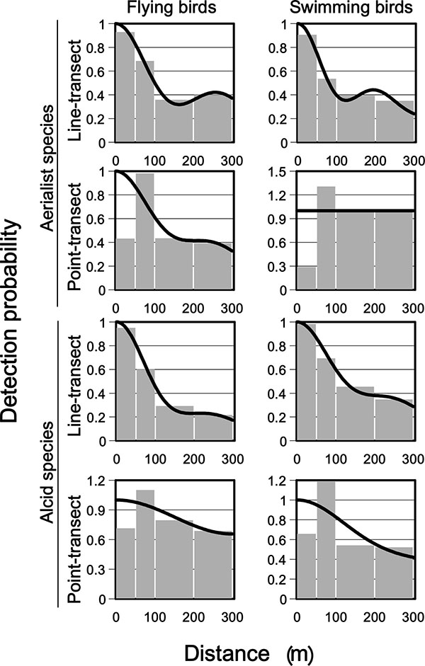 ), Table 2). The 1000 m wide line-transects provided lower detection probabilities (P) than 300 m wide line-transects (0.17-0.23 as compared to 0.43-0.55, Table 2). Uncertainty (percent CV) was generally larger in 300-m-wide transects than in 1000 m wide ones, but for flying aerialists (2-51%, and 12-21% respectively, Table 2). Differences in density estimates were generally below 0.19 birds/km2 between 300 and 1000 m wide line-transects (range: 0.02-0.19 birds/km2). Detection probability in the 300-1000 m interval was low for all groups (0.02-0.09), except for flying alcids (0.264, Table 2). The latter potentially is related to the detection of evading alcids far ahead of the ship.


Goodness of fit of detection functions for point-transects were generally poor (Fig. (1), Table 2). For all survey types, detection probability histograms suggested evasive movements within the 0-50 m interval, whereas detection probability remained relatively high out to 300 m in most cases, especially for flying alcids and swimming aerialists (Fig. 1). This made modeling of detection probability for point-transects difficult (Table 2).

Truncation distance (w), number of detections (n), detection probability beyond 300 m, fitted detection model, goodness of fit assessment (see Methods), detection probability (P, with its % CV), and difference in density estimates and coefficient of variation between 300 m and 1000 m wide line-transects, by survey type, species and behavior group for data collected during five seabirds at-sea surveys in the Gulf of St. Lawrence in 2009 and 2010. Goodness of fit statistics were classified as poor (α < 0.05) and good otherwise.
Comparison of Density Estimates
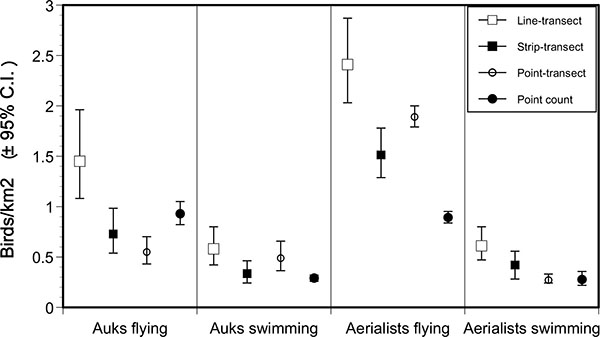
In concurrence with the above results, we used a truncation distance of 300 m for all survey types, species and behavior groups for comparison of densities among methods. Line-transect density estimates exceeded those from point-transects by a factor of 1.2 to 2.6, and the former were significantly higher in all bird groups, except for swimming alcids (Fig. 2 ). Point-transect density estimates were lower or similar to those from strip-transect and point count methods in three cases (Fig. 2).
Comparison of Coefficients of Variation Associated with Density Estimates
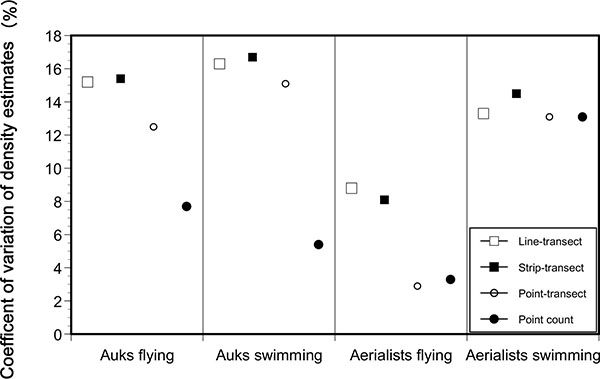
Percent CV for density estimates using line-transects varied between 8.8 and 16.3% among bird groups, whereas it ranged between 2.9 and 15.1% using point-transects (Fig. 3 ). The difference in % CV between line-transect and point-transect methods varied between 0.2 and 5.9%.
Probability of Detection Forward within the 0-50 m Perpendicular Interval
Best models of detection probability for detections forward of the vessel within the first 50 m perpendicular interval, by behavior and species predicted an overall detection probability > 0.92 in this first interval within 300 m ahead, but 0.43-0.48 within 1000 m ahead in three behavior and species classes out of four, as detection probability dropped sharply after 300 m (Fig. 4 ). However, even best models of detection functions within this interval provided poor fits caused by the lower number of observations within the first 50 m ahead (Fig. 4).
DISCUSSION
Addition of a 300-1000 m Interval
We found no evidence that the addition of a 300-1000 m interval on transects would improve modeling of the detection probability, provide different density estimates, or increase precision of these estimates. Still, the use of a 300-1000 m interval has advantages, such as discouraging observers from heaping detections beyond 300 m into the 200-300 m interval, and allowing for more detections of rare species within the survey, which may help in computing densities of such species. Yet, with detection probabilities below 0.1 beyond 300 m, these few detections will not likely be helpful and will make detection functions harder to fit [9Buckland ST, Anderson DR, Burnham KP, Laake JL, Borshers DL, Thomas L. Introduction to distance sampling. New York: Oxford University Press 2001.] and it is recommended to choose the truncation distance, w, such that g(w) ≈ 0.15 (Buckland et al. 2001, p. 135). Hyrenbach et al. [23Hyrenbach KD, Henry MF, Morgen KH, Welch DW, Sydeman WJ. Optimizing the width of strip transects for seabird surveys from vessels of opportunity. Mar Ornithol 2007; 35: 29-37.] found that detection as well as identification to species generally declined beyond 400 m. We conclude that a transect width of 1000 m generally is not warranted unless there are specific species for which it is suspected this could help. Time spent looking beyond 300 m could be better spent to help obtain more detections within the 300 m transect and along the transect line.
Strip-Transect vs. Line-Transect
Although this study did not specifically aim at comparing these two methods, it is worth mentioning that line-transects provided higher density estimates compared to strip-transects, as detection probabilities declined rapidly with distance, and were below 0.5 beyond 100 m. This pattern was similar across species classes and behavior. Although line-transects may be not practical where seabird density is high [23Hyrenbach KD, Henry MF, Morgen KH, Welch DW, Sydeman WJ. Optimizing the width of strip transects for seabird surveys from vessels of opportunity. Mar Ornithol 2007; 35: 29-37.], it is possible (and methodologically acceptable) to measure distances to a subset of birds under such conditions [9Buckland ST, Anderson DR, Burnham KP, Laake JL, Borshers DL, Thomas L. Introduction to distance sampling. New York: Oxford University Press 2001.]. The extent of the difference between the two methods varied by species and behavior, and may lead to incorrect conclusions concerning the importance of a given species in the local landscape and seabird communities. Line-transect techniques will also help when comparing among surveys since detection functions may vary among observers, periods, etc. Our results show that computation and incorporation of detection probability into density estimates is necessary for both swimming and flying birds. Granted, higher densities do not mean unbiased densities, but the clear decrease in detection beyond 100 m suggests that the line-transect method is a far better tool.
Line-Transect vs. Point-Transect
Our results suggest that the strong evasive movement of both swimming / flying alcids and aerialists precludes using the point transect method since it makes modeling the detection function problematic at best. Resulting density estimates from point-transects generally were similar to those obtained using strip-transect or point count methods, and thus provided underestimated densities as compared to the line-transect method. Estimates obtained using the line-transect method apparently still suffer from this evasive movement within the first 50 m forward in the first interval, suggesting that g(0) also remains underestimated with this method, however this can only be confirmed with mark-recapture distance sampling [24Laake JL, Borchers DL. Methods for incomplete detection at distance zero. In: Advanced Distance Sampling. Oxford University Press 2004; pp. 108-89.
]. Point-transects had greater precision than line-transects in some cases, but the underestimation of density wastoo substantial to be deemed reliable. Further, we consider that % CV of line-transects still were within acceptable limits, below 17%.
CONCLUSION
We conclude that line transects are superior to point-transects for both swimming and flying birds, and that using 300 m wide line-transects is superior to 1000 m wide transects in our area due to low detection probability beyond 300 m.
CONFLICT OF INTEREST
The authors confirm that this article content has no conflict of interest.
ACKNOWLEDGEMENTS
We are sincerely grateful to Olivier Barden and Samuel Denault for their help during fieldwork. We thank Steve T. Buckland and Carina Gjerdrum for their comments on an earlier version of this manuscript. Donna Goodwin kindly proofread an earlier version of this manuscript.
REFERENCES
| [1] | North American Waterfowl Management Plan. In: Plan Committee North American Waterfowl Management Plan 2004 Strategic Guidance: Strengthening the Biological Foundation Canadian Wildlife Service, US Fish and Wildlife Service, Secretaria de Medio Ambiente y Recursos Naturales 2004. |
| [2] | Vosta M. Global changes and new trends within the territorial structure of the oil, gas and coal industries. Acta Oeconomic Pragen 2009; 2009(1): 45-59. [http://dx.doi.org/10.18267/j.aop.3] |
| [3] | Dalsøren SB, Eide MS, Myhre G, Endresen O, Isaksen IS, Fuglestvedt JS. Impacts of the large increase in international ship traffic 2000-2007 on tropospheric ozone and methane. Environ Sci Technol 2010; 44(7): 2482-9. [http://dx.doi.org/10.1021/es902628e] [PMID: 20210355] |
| [4] | Musial W, Ram B. Large-scale offshore wind power in the United States: Assessment of opportunities and barriers National Renewable Energy Laboratory. Colorado, US: Department of Energy 2010. |
| [5] | Grecian WJ, Witt MJ, Attrill MJ, et al. A novel projection technique to identify important at-sea areas for seabird conservation: An example using the Northern gannets breeding in the North East Atlantic. Biol Conserv 2012; 156: 43-52. [http://dx.doi.org/10.1016/j.biocon.2011.12.010] |
| [6] | Montevecchi WA, Hedd A, McFarlane Tranquilla L, et al. Tracking seabirds to identify ecologically important and high risk marine areas in the western North Atlantic. Biol Conserv 2012; 156: 62-71. [http://dx.doi.org/10.1016/j.biocon.2011.12.001] |
| [7] | Tasker ML, Jones PH, Dixon T, Blake F. Counting seabirds at sea from ships: A review of methods employed and a suggestion for a standardized approach. Auk 1984; 101: 567-77. |
| [8] | Komdeur J, Bertelsen J, Cracknell G. Manual for aeroplan and ship surveys of waterfowl and seabirds, Slimbridge: IWRB Special Publication 1992. |
| [9] | Buckland ST, Anderson DR, Burnham KP, Laake JL, Borshers DL, Thomas L. Introduction to distance sampling. New York: Oxford University Press 2001. |
| [10] | Camphuysen CJ, Fox AD, Leopold MF, Petersen IK. Towards standardized seabirds at-sea census techniques in connection with environmental impact assessments for offshore wind farms in the U.K: A comparison of ship and aerial sampling methods for marine birds, and their applicability to offshore wind farm assessments. Texel 2004; pp. 37. |
| [11] | Gjerdrum C, Fifield DA, Wilhelm S. Eastern Canada seabirds at-sea (ECSAS) standardized protocol for pelagic seabird surveys from moving and stationary platforms, Technical Report Series. Canad Wildlife Serv 2012. |
| [12] | Spear LB, Nur N, Ainley DG. Estimating absolute densities of flying seabirds using analyses of relative movements. Auk 1992; 109: 385-9. [http://dx.doi.org/10.2307/4088211] |
| [13] | Bardraud C, Thiebot JB. On the importance of estimating detection probabilities from at-sea surveys of flying seabirds. J Avian Biol 2009; 40: 584-90. [http://dx.doi.org/10.1111/j.1600-048X.2009.04653.x] |
| [14] | Bolduc F, Desbiens A. Delineating distance intervals for ship-based seabird surveys. Waterbirds 2010; 34: 253-7. [http://dx.doi.org/10.1675/063.034.0216] |
| [15] | Heinemann D. A range finder for pelagic bird censusing. J Wildl Manage 1981; 45: 489-93. [http://dx.doi.org/10.2307/3807930] |
| [16] | Buckland ST. Point transect surveys for songbirds: Robust methodologies. Auk 2007; 123: 1-13. |
| [17] | Van Der Meer J, Camphuysen CJ. Effect of observer differences on abundance estimates of seabirds from ship-based strip transect surveys. Ibis 1996; 138: 433-7. [http://dx.doi.org/10.1111/j.1474-919X.1996.tb08061.x] |
| [18] | Fifield DA, Lewis KP, Gjerdrum C, Robertson GJ, Wells R. Offshore seabird monitoring program. Environ Stud Res Funds Rep 2009; 183: 68. |
| [19] | Maclean IM, Rehfisch MM, Skov H, Thaxter CB. Evaluating the statistical power of detecting changes in the abundance of seabird at sea. Ibis 2012; 155: 113-26. [http://dx.doi.org/10.1111/j.1474-919X.2012.01272.x] |
| [20] | Thomas L, Laake J, Rexstad E, et al. Disatance 60, Release 2 research unit for wildlife population assessment, University of St Andrews, UK 2009. (http://www.ruwpa.st-and.ac.uk/distance/) |
| [21] | Marques TA, Thomas L, Fancy SG, Buckland ST. Improving estimates of bird density using multiple-covariate distance sampling. Auk 2007; 124: 1229-43. [http://dx.doi.org/10.1642/0004-8038(2007)124[1229:IEOBDU]2.0.CO;2] |
| [22] | Ronconi RA, Burger AE. Estimating seabird densities from vessel transects: Distance sampling and implications for strip transects. Aquat Biol 2009; 4: 297-309. [http://dx.doi.org/10.3354/ab00112] |
| [23] | Hyrenbach KD, Henry MF, Morgen KH, Welch DW, Sydeman WJ. Optimizing the width of strip transects for seabird surveys from vessels of opportunity. Mar Ornithol 2007; 35: 29-37. |
| [24] | Laake JL, Borchers DL. Methods for incomplete detection at distance zero. In: Advanced Distance Sampling. Oxford University Press 2004; pp. 108-89. |