- Home
- About Journals
-
Information for Authors/ReviewersEditorial Policies
Publication Fee
Publication Cycle - Process Flowchart
Online Manuscript Submission and Tracking System
Publishing Ethics and Rectitude
Authorship
Author Benefits
Reviewer Guidelines
Guest Editor Guidelines
Peer Review Workflow
Quick Track Option
Copyediting Services
Bentham Open Membership
Bentham Open Advisory Board
Archiving Policies
Fabricating and Stating False Information
Post Publication Discussions and Corrections
Editorial Management
Advertise With Us
Funding Agencies
Rate List
Kudos
General FAQs
Special Fee Waivers and Discounts
- Contact
- Help
- About Us
- Search


The Open Petroleum Engineering Journal
(Discontinued)
ISSN: 1874-8341 ― Volume 12, 2019
Models for Calcium Carbonate Precipitation in the Near-Well Zone by Degassing of CO2
Magnus Wangen*, Jan Sagen, Tor Bjørnstad, Harald Johansen, Alban Souche
Abstract
Calcium carbonate scale formation is a well known problem for water producing wells. Although there are several types of scale forming processes, we investigate the case of calcium carbonate precipitation when the degassing of CO2 causes the calcium equilibrium concentration to decrease towards a production well. We study a simplified system of carbonate chemistry, which allows for analytical expressions for the porosity loss as a function of time. The precipitation process normally goes from flow-limited away from the well to precipitation-limited close to the well. We derive an expression that estimates the transition zone between these two regimes. Furthermore, we present analytical estimates for the porosity reduction at a given radius as a function of time, including an estimate for each of these precipitation regimes. These analytical results are tested against numerical solutions for the porosity loss, which account for the full set of equations of the model. The analytical models give an accurate estimate of the linear porosity reduction with time, until at least half the porosity is lost. Examples of scale formation are given for the two regimes. Reasonable values for the precipitation kinetics indicate that most production operations have a kinetics-limited regime close to the well. The models also show that this type of scale formation takes place very close to the wells, typically within a few well radii from the walls of the well.
Article Information

Identifiers and Pagination:
Year: 2016Volume: 9
First Page: 178
Last Page: 194
Publisher Id: TOPEJ-9-178
DOI: 10.2174/1874834101609160178
Article History:
Received Date: 12/12/2015Revision Received Date: 17/03/2016
Acceptance Date: 20/05/2016
Electronic publication date: 30/08/2016
Collection year: 2016
open-access license: This is an open access article licensed under the terms of the Creative Commons Attribution-Non-Commercial 4.0 International Public License (CC BY-NC 4.0) (https://creativecommons.org/licenses/by-nc/4.0/legalcode), which permits unrestricted, non-commercial use, distribution and reproduction in any medium, provided the work is properly cited.
* Address correspondence to this author at the Institute for Energy Technology P.O.Box 40, N-2027 Kjeller, Norway; Tel: +47-4767-9534; E-mail: Magnus.Wangen@ife.no
| Open Peer Review Details | |||
|---|---|---|---|
| Manuscript submitted on 12-12-2015 |
Original Manuscript | Models for Calcium Carbonate Precipitation in the Near-Well Zone by Degassing of CO2 | |
1. INTRODUCTION
“Scale” formation is the precipitation of a solid mineral from a brine [1G. Atkinson, and M. Mecik, "The chemistry of scale prediction", J. Petrol. Sci. Eng., vol. 17, pp. 113-121, 1997.
[http://dx.doi.org/10.1016/S0920-4105(96)00060-5] ]. The production of water in petroleum wells with a high water cut or brine production from geothermal wells often leads to scale formation in the near-well area [2A. Satman, Z. Ugur, and M. Onur, "The effect of calcite deposition on geothermal well inflow performance", Geothermics, vol. 28, pp. 425-444, 1999.
[http://dx.doi.org/10.1016/S0375-6505(99)00016-4] -5K. Kodel, P. Andrade, J. Valença, and N. Souza, "Study on the composition of mineral scales in oil wells", J. Petrol. Sci. Eng., vol. 81, pp. 1-6, 2012.
[http://dx.doi.org/10.1016/j.petrol.2011.12.007] ]. EOR operations with CO2 injection will likely lead to scale formation, especially for fields with a history of water injection prior to CO2 injection. There are at least two different types of processes that cause scale formation. One process is the mixing of incompatible formation waters from different parts of a reservoir, such as the mixing of barium brine with sulfate rich brine, as they approach the production well. This mixing leads to the formation of barium sulfate scale. The other process of scale formation results from a reduction in the equilibrium concentration of mineral forming ions in the brine as they approaches the production well. A decreasing equilibrium concentration is typically caused by a reduction in the fluid pressure. It is the latter process we study here, i.e. when the brine is produced together with a gas phase rich in CO2. We present models for the loss of porosity caused by calcium carbonate scale formation, when the brine pressure and the partial pressure of CO2 decrease towards a production well.
The clogging of the near-well area of a production well with calcium carbonate is a multi-phase flow process, whereby the mineral precipitates from a brine containing a number of salt-forming cations and anions. The precipitation is controlled by the super-saturation of calcium bearing minerals and by the kinetics of the precipitation. At the same time, the absolute permeability decreases as a result of the reduction in porosity.
In order to treat this process analytically we need to make some simplifications. The model assumes that the water phase is saturated with CO2 and that it is in contact with a CO2 dominated gas phase. The case where the water phase is not saturated with CO2 may not necessarily lead to scaling and is, therefore, not a part of this study. An oil phase could be present, but the rock surface needs to be in contact with the water phase for fluid-rock reactions to occur. The degassing of CO2 from the water phase takes place as the fluid pressure decreases towards the production well. It is assumed that the capillary pressure difference between the water phase and the gas phase is negligible. Since the gas phase is dominated by CO2 we approximate the partial pressure of CO2 in the gas phase with the pressure of the water phase. By assuming the reservoir rock is initially saturated with the water phase, the relative permeability of the water phase decreases from 1 with an increase in the gas phase. Assuming that water phase occupies most of the pore space, we approximate the relative permeability of the gas phase to be 1. A value less than one could have been used, but considering the uncertainty associated with the absolute permeability we use the value of 1 for simplicity. We assume a simple brine with dissolved CO2 and CO2+. This approach is similar to that of Satman et al. [2A. Satman, Z. Ugur, and M. Onur, "The effect of calcite deposition on geothermal well inflow performance", Geothermics, vol. 28, pp. 425-444, 1999.
[http://dx.doi.org/10.1016/S0375-6505(99)00016-4] ], where they also assume that the partial pressure of the CO2 is the same as the pressure of the water phase. Satman et al. [2A. Satman, Z. Ugur, and M. Onur, "The effect of calcite deposition on geothermal well inflow performance", Geothermics, vol. 28, pp. 425-444, 1999.
[http://dx.doi.org/10.1016/S0375-6505(99)00016-4] ] assumed that the relative permeability of the water phase decreased as the gas saturation increased with the liberation of CO2 from the brine, while keeping the fluid pressure and the fluid pressure gradient constant. Here we make an alternative assumption that relative permeability of water phase remains close to 1, while the absolute permeability changes with the clogging of the pore space. Therefore, we consider a simple water dominated system in equilibrium with a CO2 gas phase at low saturation.
The reservoir rock is assumed to contain both calcite and aragonite, and to be initally in equilibrium with the brine. Even though we consider a relatively simple system, we think that much of what we can learn from it is useful for more complex systems. The modelling we present here bridges numerical simulations of laboratory experiments over days with near-well predictions on a time scale of years [6S. Hassfjell, A. Haugan, and T. Bjørnstad, "“47Ca-aided studies of CaCO3 scaling rates at low saturation ratios", Soc. Pet. Eng. SPE, vol. 121441, pp. 1-18, 2009., 7E. Stamatakis, A. Stubos, and J. Muller, "Scale prediction in liquid flow through porous media: A geochemical model for the simulation of caco3 deposition at the near-well region", J. Geochem. Explor., vol. 108, pp. 115-125, 2011.
[http://dx.doi.org/10.1016/j.gexplo.2010.11.004] ]. It should be mentioned that calcite precipitation by degassing is a common process in nature [8W. Dreybrodt, D. Buhmann, J. Michaelis, and E. Usdowski, "Geochemically controlled calcite precipitation by CO2 outgassing: Field measurements of precipitation rates in comparison to theoretical predictions", Chem. Geol., vol. 97, pp. 285-294, 1992.
[http://dx.doi.org/10.1016/0009-2541(92)90082-G] ].
Roberts [9B. Roberts, "The effect of sulfur deposition on gaswell inflow performance", SPE Reservoir Eng, vol. 12, no. 2, pp. 118-123, 1997.] and Satman et al. [2A. Satman, Z. Ugur, and M. Onur, "The effect of calcite deposition on geothermal well inflow performance", Geothermics, vol. 28, pp. 425-444, 1999.
[http://dx.doi.org/10.1016/S0375-6505(99)00016-4] ] both assumed that the kinetics of the calcium carbonate precipitation is sufficiently fast for the concentration of calcium ions to be close to the equilibrium concentration all the way to the well. This equilibrium assumption simplifies the modelling, because the calcium ion concentration is then obtained from knowledge of the fluid pressure. The Darcy flux increases towards the production well as 1/r, where r is the radius from the center of the well. Close to the well the Darcy flux may easily become too large for the precipitation rate to keep the calcium ion concentration close to its equilibrium value. It is uncertain if the assumption of equilibrium is sound in the near well area. It is therefore reasonable to expect that there is a transition from a regime away from the well, where flow is the rate limiting process, to a regime close to the well, where kinetics becomes the rate limiting process. Here we derive an expression for the position where the flow-limited regime ends and the kinetics-limited regime begins. The estimate is based on a solution of the stationary convection-reaction equation, which is a special case of the full non-linear convection-diffusion equation for geochemical modelling [10P. Lichtner, "The quasi-stationary state approximation to coupled mass transport and fluid-rock interaction in a porous medium", Geochim. Cosmochim. Acta, vol. 52, no. 1, pp. 143-165, 1988.
[http://dx.doi.org/10.1016/0016-7037(88)90063-4] , 11M. De Simoni, X. Sanchez-Vila, J. Carrera, and M. Saaltink, "A mixing ratios-based formulation for multicomponent reactive transport", Water Resour. Res., vol. 43, no. W07419, pp. 1-10, 2007.
[PMID: 20300476] ]. Mineral precipitation behaves differently in the two regimes of scale formation described above. We derive analytical expressions for the porosity loss at a given radius as a function of time for scale formation in both regimes. These expressions are tested by comparing them with numerical solutions.
The paper is organized as follows: The basic equations behind the scale formation model are presented, followed by a short resume is of calcium carbonate equilibrium. Then, a derivation is given for the position of the transition zone between the flow-limited and the precipitation-limited regimes. Finally, analytical expressions for the porosity evolution are formulated and demonstrated for both regimes.
2. THE BASIC EQUATIONS IN THE MODEL OF SCALE FORMATION
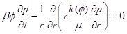
Our aim is to model calcium carbonate scale formation driven by a decrease in the equilibrium concentration of calcium ions towards the production well. We assume that the gas phase is dominated by CO2 and that the water saturation is much higher than the gas saturation. Furthermore, we assume that the capillary pressure between the gas phase and the water phase is negligible, implying that the gas pressure is the same as the brine pressure. The model then involves three main equations. The first is the pressure equation in cylinder coordinates
 |
(1) |
for a horizontal aquifer with constant thickness and radial symmetry around the well. The radius is r, β is the effective compressibility, µ is the viscosity and k(Ø) is the absolute permeability as a function of porosity ϕ given as
 |
(2) |
where k 0 is the initial permeability and ϕ 0 is the initial porosity. The exponent n controls how the permeability depends on the porosity, where n=3 corresponds to the Kozeny-Carman model. The exponent n may take different values for different types of rocks [12M. Wangen, Physical Principles of Sedimentary Basin Analysis., Cambridge University Press: UK, 2010.
[http://dx.doi.org/10.1017/CBO9780511711824] ]. Boundary conditions for the pressure equation (1) is a constant well pressure at the well radius rw and a constant pressure pmax at a distant radius rmax. We assume that the system stays close to a stationary state, which is likely the case for geothermal systems operated with a fixed injection and production pressures, as well as for oil and gas producing wells with a high water-cut maintained by pressure support from water injection at constant pressure. The numerical solution of pressure equation (1) is initialized with a stationary reservoir pressure. The solution for the fluid pressure (1) gives the Darcy flux
 |
(3) |
which is important for the transport of ions. The transport-reaction equation for calcium ions is [10P. Lichtner, "The quasi-stationary state approximation to coupled mass transport and fluid-rock interaction in a porous medium", Geochim. Cosmochim. Acta, vol. 52, no. 1, pp. 143-165, 1988.
[http://dx.doi.org/10.1016/0016-7037(88)90063-4] ]
 |
(4) |
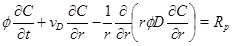
where the calcium ion concentration is denoted as C. The left-hand-side expresses the transport of calcium ions by means of advection with a radial Darcy flux, vD, towards the well and by diffusion with diffusivity, D. The right-hand-side of equation (4) is the precipitation rate [10P. Lichtner, "The quasi-stationary state approximation to coupled mass transport and fluid-rock interaction in a porous medium", Geochim. Cosmochim. Acta, vol. 52, no. 1, pp. 143-165, 1988.
[http://dx.doi.org/10.1016/0016-7037(88)90063-4] , 13P. Aagaard, and H. Helgeson, "Thermodynamic and kinetic constrains on reaction-rates among minerals and aqueous solutions 1. theoretical considerations", Am. J. Sci., vol. 282, no. 3, pp. 237-285, 1982.
[http://dx.doi.org/10.2475/ajs.282.3.237] ].
 |
(5) |
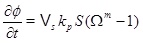
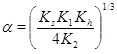
The precipitation rate Rp is proportional to the reaction constant kp, the specific surface area S of the pore space and the difference from equilibrium expressed by the saturation index W given as
 |
(6) |
The exponent m takes values from around 1 to more than 3 for different precipitation modes [14C. Noiriel, C. Steefel, L. Yang, and J. Ajo-Franklin, "Upscaling calcium carbonate precipitation rates from pore to continuum scale", Chem. Geol., vol. 318-319, pp. 60-74, 2012.
[http://dx.doi.org/10.1016/j.chemgeo.2012.05.014] ]. We let m=1 as suggested by Stamatakis et al. [7E. Stamatakis, A. Stubos, and J. Muller, "Scale prediction in liquid flow through porous media: A geochemical model for the simulation of caco3 deposition at the near-well region", J. Geochem. Explor., vol. 108, pp. 115-125, 2011.
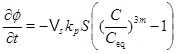
[http://dx.doi.org/10.1016/j.gexplo.2010.11.004] ]. Both the surface area, S, and the diffusivity, D, will decrease as the porosity decreases. These effects are not accounted for and the modelling is, therefore, less reliable for a substantial loss in porosity. Boundary conditions for the concentration equation (4) are the equilibrium of calcium ions and a zero gradient at the outer boundary (r=rmax). The reaction term in the concentration equation gives the rate of calcium ions that precipitates from the brine. The time-rate of change of porosity is proportional to the precipitation rate (5), and is
 |
(7) |
where Vs is the molar volume of calcite. The pressure equation (1), the concentration equation (4) and the porosity equation (7) form the basis for the modelling of scale formation. The numerical solutions have as initial conditions a steady state pressure and concentration. The equations are solved numerically in a sequential manner, by first solving for pressure, then for concentration, and finally for porosity. The pressure dependent equilibrium concentration is updated before the concentration equation is solved, and the permeability is updated with the porosity after a new time step. Both the pressure and concentration equation are solved with an implicit standard finite difference scheme, where the reaction term is linearized and taken implicitly. The equilibrium concentration of calcium ions and other aqueous species are also a part of the model. The next section explains how the equilibrium concentration and the saturation index are computed.
3. CALCIUM CONCENTRATION IN THE BRINE
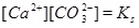
It is assumed that the aqueous CO2 is in equilibrium with a CO2 gas phase. The capillary pressure between the brine and the gas phase is assumed to be negligible and the partial pressure of CO2 is therefore assumed to be the same as the fluid pressure. Although the ions in the brine have an effect on the ionic strength, it is simply assumed that the activity coefficients are equal to one. CO2 will initially be in a supercritical state if pressure and temperature are beyond the critical point. There are 6 unknown aqueous species to be solved for in the aqueous system, which is made as simple as possible
 |
(8) |
Equilibrium is expressed by the following five reactions [15W. Stumm, and J. Morgan, Aquatic Chemistry., John Wiley & Sons, Inc.: US, 1996.],
 |
(9) |
where the equilibrium constants are shown in the column to the right. The corresponding mass action laws and the expression of electro neutrality are given as follows
 |
(10) |
 |
(11) |
 |
(12) |
 |
(13) |
 |
(14) |
 |
(15) |
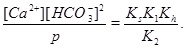
A numerical solution of these equations is shown in Fig. (1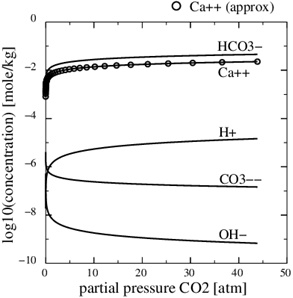 ), which shows the calcium concentrations as a function of the partial pressure of CO2 at the temperature T=20 °C. Recall that the CO2-pressure is taken to be equal to fluid pressure, p, and we therefore have that the carbonic acid is proportional to the fluid pressure. It is seen from the charge balance that [HCO-3] is close to 2[Ca2+], since these two concentrations dominate. This approximation is reasonable in the acidic regime, which applies when CO2 is dissolved in the water phase. The use of [HCO-3]≈[Ca2+] allows for an approximate expression for [Ca2+] as a function of fluid pressure. The equilibrium expressions from (12) to (14) can be combined into the following expression for [Ca2+]
 |
(16) |
by inserting [H+] from equation (12) into equation (13), which then gives [CO2-3] expressed with [HCO-3]. The approximation 2[Ca2+]≈[HCO-3] then leads to [15W. Stumm, and J. Morgan, Aquatic Chemistry., John Wiley & Sons, Inc.: US, 1996.]
 |
(17) |
where
 |
(18) |
and where the mass-action constants Kh, K1, K2, Kw and Ks depend on temperature. The temperature dependence of the mass-action K-functions is found in the Appendix. This is a simple expression between the calcium equilibrium concentration and the fluid pressure, which is sufficiently accurate considering other uncertainties like reservoir permeability and precipitation rate. The solubility (17) is in agreement with the correlation used by Satman et al. [2A. Satman, Z. Ugur, and M. Onur, "The effect of calcite deposition on geothermal well inflow performance", Geothermics, vol. 28, pp. 425-444, 1999.
[http://dx.doi.org/10.1016/S0375-6505(99)00016-4] ], which covers a pressure up to 6 MPa. In addition to the calcium ion concentration, we can also express the concentration of the other species, in particular [H+], as a function of pressure [15W. Stumm, and J. Morgan, Aquatic Chemistry., John Wiley & Sons, Inc.: US, 1996.].
 |
Fig. (1) The Ca2+-concentration in the aqueous phase as a function of the partial pressure of CO2. The analytical concentration (17) is shown by the circular markers. |
It is not always possible to assume equilibrium when both reaction and transport take place. However, the carbonate species are assumed to be in equilibrium and the mass action laws (10) to (14) apply together with electro neutrality (15). The difference introduced by kinetics is that the mass action law for calcium equilibrium is replaced by a precipitation rate for calcite. The precipitation rate depends on by how much the saturation index (6) exceeds one. The saturation index can be rewritten as
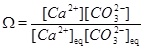 |
(19) |
where the mass action constant Ks is replaced by the product of the equilibrium concentrations of Ca2+ and CO2-3. We can express the saturation index in terms of calcium ion concentrations by first using the two mass action laws (12) and (13) to replace [CO2-3] by [HCO-3]2. These mass action laws apply both for the equilibrium and the non-equilibrium state. From electro neutrality we have the approximation 2[Ca2+]≈[HCO-3], which then gives
 |
(20) |
where Ceq is the calcium equilibrium concentration. The reaction-transport equation (4) for calcium ions is then decoupled from CO2-3 and the other aqueous species.
4. SLOW OR FAST KINETICS RELATIVE TO TRANSPORT
The Darcy flux increases towards the well proportional to 1/r in a sealed horizontal aquifer, when the pressure field is stationary. The 1/r dependency gives a steep increase in the Darcy flux close to the well. The calcium ion concentration stays close to equilibrium as long as the Darcy flow is “slow”, meaning that the precipitation kinetics keep pace with the Darcy flux. In this case, it is straightforward to compute the amount of calcite that precipitates from knowledge of the equilibrium concentration. Since we cannot be sure that the system is in equilibrium close to well, we need to decide in which regime we are at a certain distance from the well; equilibrium or non-equilibrium. We can derive a condition for when a near equilibrium condition prevails, starting from the reaction-transport equation for the Ca2+-ions.
It is therefore assumed that the reaction and transport are in a stationary state and that diffusion is negligible relative to convection. An eventual transient phase leading to the stationary state is assumed to be less important. The reaction-transport equation (4) then reduces to
 |
(21) |
The volume production rate Q gives that the radial Darcy flux vD under stationary conditions is
 |
(22) |
where h is the thickness of the aquifer. Although equation (21) looks simple, it appears to be difficult to solve it analytically, because of the non-linearity in C combined with the dependency of vD on r. Fortunately, a solution of the linear equation (for m=1/3) is useful and can be used to approximate the solution for m=1 by increasing the reaction rate by a factor of 3. The assumption that m=1 is therefore the value that is used in the numerical solutions. The analytical treatment of the case using m=1 is based on expressions for m=1/3 and a reaction rate that is 3 times faster. A dimensionless version is obtained by introducing the dimensionless radius ȓ=r/r 0 and dimensionless calcium concentration Ĉ=C/C 0, where r 0 and C 0 are the characteristic length and concentration of the system, respectively. The reaction transport equation (21) for m=1/3 becomes
 |
(23) |
where Ĉeq=Ceq/C 0 and N is the Damköhler-number
 |
(24) |
with respect to the characteristic radius r 0, and where v 0 is the Darcy flux at distance r 0 [16C. Steefel, Geochemical Transport and Kinetics., Springer: Germany, 2008, pp. 545-589.]. The Damköhler-number N is a measure of the reaction rate relative to the convective mass transport rate [16C. Steefel, Geochemical Transport and Kinetics., Springer: Germany, 2008, pp. 545-589.]. Reaction dominates transport when the Damköhler-number is much larger than 1, and the reaction rate is sufficiently fast to bring the calcium concentration to almost equilibrium. In the opposite regime, transport by convection dominates reaction, and the supersaturated fluid moves through the system too fast to experience noticeable reaction. The definition of the Damköhler-number shows that the Damköhler-number increases away from the well with the characteristic distance r2 0. This dependence on distance reflects the decrease in the Darcy flux with an increasing radius in cylinder coordinates. The dimensionless reaction-convection equation (23) has the solution for the calcium ion concentration
 |
(25) |
where Ĉin is the calcium concentration at radius r 0 (ȓ=1). In other words, Ĉin is the boundary condition at the entrance of the radial domain from r 0 to rw. Solution (25) shows the expected behaviour of the model in terms of the Damköhler-number, N. Reaction kinetics are fast relative to flow when N>>1, and the concentration (25) thus becomes close to the equilibrium concentration, Ĉ≈Ĉeq. The other regime (N<<1), where the reaction is slow relative to flow, results in the concentration (25) becoming close to the input concentration, Ĉ≈Ĉin. This behaviour is seen in Fig. (2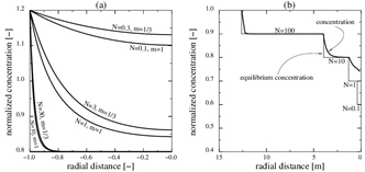 ), which compares the numerical solutions of (21) for m=1 and Damköhler-numbers N=0.1, 1 and 10 with the approximation (25). The approximation is based on m=1/3 and makes use of a Damköhler-number N that is increased by a factor of 3. The stationary concentration equation (21) is solved numerically using up-stream discretization and Newton’s method to handle the non-linearities in the reaction term.

Calcite scale formation is driven by an equilibrium concentration that decreases towards the well due to a decreasing fluid pressure. We can use equation (23) to find the solution for the case of a step-wise decrease in the equilibrium concentration by chaining together a series of solutions (25); each with a proper characteristic length.
From the definition of the Damköhler-number it follows that there is a distance rN=r(N) for each number N. We will now look at an example that has Ĉin=Ĉeq=1 for r>r(N=100). In this case, the characteristic concentration C 0 is, therefore, the equilibrium concentration for r>r100. The dimensionless equilibrium concentration drops as a piece-wise constant as follows
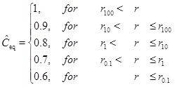 |
(26) |
The solution for the concentration is split into different intervals, with different constant equilibrium concentrations. The input concentration for an interval, Ĉin, is the solution at the same position as the preceding interval. The first interval has Ĉin=1 and each interval has its own characteristic length and Damköhler-number. The solution is shown in Fig. (2). The solution is shown in Fig. (2). The interval between r(N=100) and r(N=10) is covered by the solution with N=100 and the concentration decreases to the equilibrium concentration at the beginning of the interval. In this regime flow is the rate limiting processe. The same can be said about the next interval with N=10. The interval N=1 becomes the transition between the flow-limited and the reaction-limited processes. Finally, for the interval N=0.1 reaction is clearly the rate limiting.
5. SCALE FORMATION IN THE FLOW-LIMITED REGIME
Mass conservation of calcium ions gives that the rate of change of porosity is
 |
(27) |
where Vs is the molar volume of calcite, ∂C/∂r is the calcium ion concentration gradient towards the well, and vD is the Darcy flux. Equation (27) applies regardless of whether the regime is flow-limited or precipitation-limited, since it follows directly from mass conservation. In the flow-limited regime, where N>>1, the calcium ion concentration is close to equilibrium. It is then possible to use the equilibrium concentration directly in (27) to compute the porosity change. This approach is used in the models proposed by Roberts [9B. Roberts, "The effect of sulfur deposition on gaswell inflow performance", SPE Reservoir Eng, vol. 12, no. 2, pp. 118-123, 1997.] and Satman et al. [2A. Satman, Z. Ugur, and M. Onur, "The effect of calcite deposition on geothermal well inflow performance", Geothermics, vol. 28, pp. 425-444, 1999.
[http://dx.doi.org/10.1016/S0375-6505(99)00016-4] ]. Equation (17) shows the calcium concentration as a function of the partial pressure of CO2. The pressure is assumed to be stationary, as done by Satman et al. [2A. Satman, Z. Ugur, and M. Onur, "The effect of calcite deposition on geothermal well inflow performance", Geothermics, vol. 28, pp. 425-444, 1999.
[http://dx.doi.org/10.1016/S0375-6505(99)00016-4] ], and is given in cylinder coordinates
 |
(28) |
where rw is the well radius, pw is the well pressure and Q 0 is the initial production rate. It is now straightforward to integrate equation (27) to obtain the porosity as a function of time at a given radius
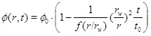 |
(29) |
where the time constant is
 |
(30) |
and the function f is
 |
(31) |
The porosity function (29) shows that the pore space at the well (r=rw) is fully clogged at time t 0. The characteristic time t 0 is similar to the time obtained by Satman et al. [2A. Satman, Z. Ugur, and M. Onur, "The effect of calcite deposition on geothermal well inflow performance", Geothermics, vol. 28, pp. 425-444, 1999.
[http://dx.doi.org/10.1016/S0375-6505(99)00016-4] ] for the complete plugging of the pore space next to the well, where their dC/dr is replaced by explicit expressions for (dC/dp)(dp/dr). Another difference is that Satman et al. [2A. Satman, Z. Ugur, and M. Onur, "The effect of calcite deposition on geothermal well inflow performance", Geothermics, vol. 28, pp. 425-444, 1999.
[http://dx.doi.org/10.1016/S0375-6505(99)00016-4] ] included a brine formation factor and a factor for the relative permeability of the water phase.
The linear decrease in the porosity with time assumes that the pressure field and flow rate remain constant. This is not the case when the porosity and the permeability approach zero. On the other hand, we expect the linear behaviour to be a useful approximation of moderate porosity reductions; for instance to half the initial porosity. The time it takes to reach the porosity ϕ1 at radius r and to clog a fraction ϕ1/ϕ 0 of the initial porosity becomes
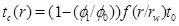 |
(32) |
Here we use the term half-life for the time needed for the initial porosity to be reduced by half (t 0/2). The porosity expression (29) can be used to estimate the width of the zone around the well where scale formation takes place. The width is defined by the radius where 5% of the porosity is lost, at the time t 0/2, which is when half the initial porosity is lost at r=rw. The solution of the equation f(r/rw)(r/rw)=10 gives that flow-limited scale formation takes place mainly in the interval
 |
(33) |
It is only a thin area around the well that becomes clogged by the precipitation process, and it is less than three times the well radius. The porosity relationship (29) can also be written in a dimensionless form using dimensionless time t=t/t 0 and dimensionless radius r=r/rw as
 |
(34) |
where the dimensionless porosity is ϕ=ϕ/ϕ 0.
Fig. (3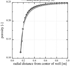 ) shows an example of calcium carbonate scale formation in the flow-limited regime (N>>1), when this regime extends all the way to the well. The curve named analytical porosity (1) is computed with equation (29) and the curve analytical porosity (2) is the same equation, but with f=1. The numerically computed porosity is also shown. The latter takes into account that the permeability decreases with decreasing porosity. Fig. (3) also shows the situation after t=4080 days, when half the numerically computed porosity is lost. The characteristic time of t 0=8833 days results in a half-life of t 0/2=4417 days, which is quite close to the numerical result. The match between the two different analytical expressions and the numerical porosity is good because in this case p 0/pw<<1, forcing the f-function (31) close to one.
 |
Fig. (3) The porosity in the flow-limited case. The markers show the position of the nodes in the numerical solution. |
The Damköhler-number N is proportional to the kinetics parameters kpS and inversly proportional to the flow rate Q 0. Fast kinetics and a low production rate assure that N>>1 and that the flow-limited regime applies for all r≥rw. The Damköhler-number is shown in Fig. (4 ). It increases by two order of magnitude from r=rw to r=10rw, because Damköhler-number is proportional to r2. Notice that parameters kpS are not included in the porosity function (29) for scale formation in this regime. The parameters used in this example are listed in Table 1.

 |
Fig. (4) The log10 (N) in the flow-limited case. The Damköhler-number is N>>1 for all r>rw. |
Fig. (5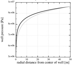 ) shows that the chosen permeability (k 0=2.10-16) results at a stationary pressure with a steep gradient towards the well. Fig. (5) also shows the numerical stationary pressure that takes into account the reduced permeability from the reduced porosity shown in Fig. (3). The numerical stationary pressure and the analytical stationary pressure are close, because the porosity is only reduced by half next to the well, which has a moderate impact on the permeability field. A decreasing permeability close to the well implies a decreasing production rate, since the well pressure and the outer boundary pressures are kept constant. In the current example, the initial production rate decreased by 30%, when the initial porosity was reduced by half.
 |
Fig. (5) The pressure in the flow-limited case. The analytical expression shows the initial pressure. The numerical pressure corresponds to the numerical porosity in Fig. (3 ), where half the porosity is lost close to the well. |
We also notice that the pressure gradient gets steeper close to the well, where the permeability is reduced, and that it gets less steep where the permeability is intact. The large pressure gradient near the well also gives a steep decline in the calcium equilibrium concentration, as seen in Fig. (6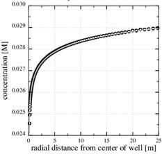 ). The continued scale formation after half the initial porosity is lost becomes progressively non-linear, and the scaling process moves towards the well since it follows the increasing pressure decline towards the well.

The porosity functions (29) and (34) do not account for the feed-back from the reduced porosity on the fluid pressure, which in turn has a feed-back on the equilibrium concentration and the scale formation rate. Nevertheless, the numerical solutions show that the linear estimate of porosity reduction is reasonably good to at least half the initial porosity. The modelling of scale formation, when porosity approaches the percolation threshold and the pore space becomes almost impermeable, is beyond the current modelling efforts.
6. SCALE FORMATION IN THE KINETICS-LIMITED REGIME
The rate of change of porosity is given by equation (27), which follows from the mass conservation of the calcium ions. This equation is useful in the flow-limited regime, where the kinetics are sufficiently fast to keep the calcium concentration close to the equilibrium. The rate of change of porosity can then be computed with only the knowledge of the equilibrium concentration.
On the other hand, in the kinetics-limited regime we need the kinetics, because we are not close to equilibrium. We can use the reaction-advection equation (21) to obtain an expression for the rate of change of porosity
 |
(35) |
The pressure dependent calcium equilibrium concentration is given by (17), but we do not know the concentration C, without a full solution for the transport-reaction equation. It is, however, possible to estimate the concentration in the regime N<<1 by using the knowledge of where the system has a transition from flow-limited to precipitation-limited. The equilibrium concentration at the radius of N=1 is a good estimate. The concentration is almost in equilibrium at the flow-limited regime (N>>1), but the kinetics cannot keep pace with the flow when the fluid approaches the well, and N becomes much less that one. The kinetics then become the rate limiting process for the interval between this radius and the well. The flow increases as 1/r towards the well and the regime becomes increasingly more kinetics-limited. The concentration at the radius of N=1 will, for this reason, not decrease much from this position during the brine’s flow towards the well. The drive for precipitation is that the fluid and CO2 pressure continue to drop towards the well, which creates an increasing super-saturation. The radius at N=1 is denoted by r1 and we therefore have
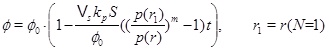 |
(36) |
after a straightforward integration in t. Expression (36) for porosity as a function of time at a given radius leads to the time needed to clog the pore space as
 |
(37) |
The time estimate is inversely proportional to the precipitation constant kp and the specific surface area S. An uncertainty of at least one order of magnitude in these two factors is more important than the error introduced by taking the equilibrium concentration at the radius of N=1 for the precipitation-limited regime.
Fig. (7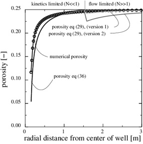 ) shows the porosity when precipitation kinetics is the rate limiting process in the near well area, while the data for the case is listed in the Table 1. The precipitation rate kp is based on data from Noiriel et al. [14C. Noiriel, C. Steefel, L. Yang, and J. Ajo-Franklin, "Upscaling calcium carbonate precipitation rates from pore to continuum scale", Chem. Geol., vol. 318-319, pp. 60-74, 2012.
[http://dx.doi.org/10.1016/j.chemgeo.2012.05.014] ] for saturation indices less than 6. The rate kpS, which includes the specific surface area of the pore space, is nearly an order of magnitude less than what was measured by Stamatakis et al. [7E. Stamatakis, A. Stubos, and J. Muller, "Scale prediction in liquid flow through porous media: A geochemical model for the simulation of caco3 deposition at the near-well region", J. Geochem. Explor., vol. 108, pp. 115-125, 2011.
[http://dx.doi.org/10.1016/j.gexplo.2010.11.004] ] for saturation indices in the range from 15 to 216. Fig. (10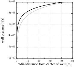 ) shows that the precipitation kinetics is the rate limiting process, because the Damköhler-number decreases towards the well and becomes 1 at the distance of r1≈2 m. The Damköhler-number decreases to much less than one from r1 until the well at rw. The same behaviour is also seen from the concentration plot shown in Fig. (9
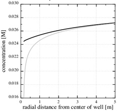 ). The calcium ion concentration is close to equilibrium until r1 is reached (N=1), but then the equilibrium concentration drops steeply towards the well and the concentration continues to decrease slightly. The porosity plotted by curve (1) in Fig. (7) is a combination of the flow-limited porosity estimate (29) and the estimate (36) for the kinetics-limited regime. The transition takes place at the radius for N=1/2, which is where there is a discontinuity in porosity. The analytical porosity curve (2) is the simplified version of expression (29) where the function f is equal to 1.
 |
Fig. (7) The porosity in the kinetics-limited case. (a) The porosity for the kinetics-limited case close to the well. (b) The porosity in the entire domain. |
The analytical approximations are very close to the numerical computed porosity, which involves a numerical solution for the fluid pressure and concentration coupled to the changing porosity. Fig. (7) shows the porosity at time t=1660 days, when the numerical porosity is reduced by half. The time scale for the kinetics gives a half-life of tk/2=1055.5, which is less than that calculated from the numerical model. The analytical estimate gives a shorter half-life than the numerical model, because it overestimates the super-saturation close to the well. It should also be mentioned that assuming a flow-limited regime near the well would strongly overestimate the rate of kinetics and strongly underestimate the porosity half-life. The half-life for the case of the flow-limited regime is t 0/2=75 days.
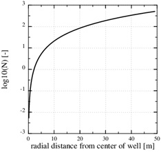 |
Fig. (8) The pressure in the kinetics-limited case. The numerical pressure corresponds to the numerical porosity in (Fig. 7 ). The analytical pressure is the same as the initial pressure. |

 |
Fig. (10) The log10 (N) in the kinetics-limited case. The transition from flow-limited to kinetics-limited regimes, defined by N=1, is at r1=2.2 m. |
The steep drop in the equilibrium concentration towards the well is a direct result of the steep pressure gradient, as seen in Fig. (8 ). The stationary numerical pressure is compared with the stationary analytical pressure, when the numerical porosity has dropped to roughly the half, and the difference is moderate.
The parameters used in this study are listed in (Table 1). The characteristic time tk is inversely proportional to the parameters for the kinetics, kp and S, which both carry large uncertainties. In addition, the initial permeability is also an important, but uncertain parameter, since it controls the fluid pressure, which in turn controls the equilibrium concentration.
This paragraph shows numerical results for the evolution of porosity, pressure and calcium ion concentration, when the porosity decreases towards zero. Fig. (11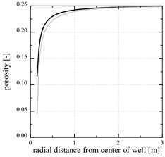 ) shows the porosity at the later time, 3790 days, when only 5% of the initial porosity is left according to the numerical simulation. The zone of scale formation has increased little in width and only the porosity very close to the well has decreased. This behaviour is caused by the decrease in the permeability near the well. The corresponding numerical fluid pressure in Fig. (12
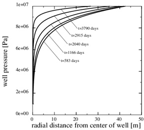 ) shows that most of the pressure drop is over the thin zone clogged with minerals. The fluid pressure, therefore, leads to a decreasing equilibrium concentration next to the well, where the porosity and permeability are lowest. The numerical calcium concentration is close to equilibrium, except for the thin zone with substantial mineral scale, as seen in Fig. (13
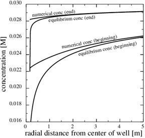 ). Fig. (14
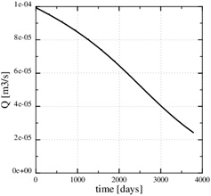 ) shows the decrease in production rate with increasing time and loss of permeability from mineral precipitation. The initial production rate has been reduced to roughly 20% of its initial value because of the scale formation, which in turn leads to an increase in the Damköhler-number. The flow-limited regime, therefore, approaches the well with increasing precipitation and loss of porosity and permeability.
 |
Fig. (11) The numerically computed porosity at the time when the initial porosity is reduced by 50% and 80%. |
 |
Fig. (12) The fluid pressure at 5 equidistant times between the beginning and the end of the simulation. The pressure gradient increases steeply over the near well area with time. |
 |
Fig. (13) The equilibrium concentration follows the fluid pressure, and it gets increasingly steep towards the well. |
 |
Fig. (14) The brine production rate decreases with time. |
CONCLUSION
We present models for the formation of calcium carbonate scale near production wells, when the produced fluid is a brine of dissolved CO2 and Ca2+. It is also assumed that the reservoir contains a minor portion CO2 rich gas, which is produced with the brine. It is the pressure drop in the gas phase that leads to a drop in the calcium equilibrium concentration in the brine, and it is the decreasing equilibrium concentration that drives the precipitation process.
Two analytical estimates for the porosity reduction are presented for this system. The first estimate applies to the regime where kinetics is sufficiently fast to keep pace with the Darcy flow, which results in the flow being the rate limiting process. The calcium concentration is also close to equilibrium in this regime. The second analytical estimate applies in the opposite regime, where kinetics is the rate liming process because it cannot keep pace with the flow. The brine is initially in the flow-limited regime far from the well, but as the flux increases towards the well, the brine will most likely at some point enter the kinetics-limited regime. We have derived an estimate for the position where the scale formation regime changes from flow-limited to kinetics-limited. The analytical results predict the porosity at any radius as a function of time. The porosity decreases linearly with time in these models. The analytical expressions for porosity and the half-life predictions are tested against numerical computations. The analytical expressions compare well with the numerical results until half the initial porosity is lost close to the well. Scale formation, when the porosity approaches the percolation threshold, however is not a part of the modelling. The half-life estimates for the porosity give an indication of how long one can expect production wells to operate before scale formation becomes a problem. The analytical expressions for scaling from a simple brine containing CO2 and Ca2+ can be a useful reference for scale formation from real brine solutions.
APPENDIX
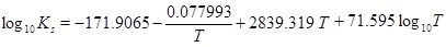
The mass-action parameters are taken from Stumm and Morgan [15W. Stumm, and J. Morgan, Aquatic Chemistry., John Wiley & Sons, Inc.: US, 1996.], where the temperature is in Kelvin and the pressure that is multiplied with Kh is in units atm.
 |
 |
 |
 |
 |
CONFLICT OF INTEREST
The authors confirm that this article content has no conflict of interest.
ACKNOWLEDGEMENTS
This work has been partially funded by the SUCCESS center for CO2 storage under grant 193825/S60 from Research Council of Norway (RCN). SUCCESS is a consortium with partners from industry and science, hosted by Christian Michelsen Research AS. The authors are greatful for the comments and suggestions of two anonymous referees and to Kristin Mueller for her assistance with the English.
REFERENCES
| [1] | G. Atkinson, and M. Mecik, "The chemistry of scale prediction", J. Petrol. Sci. Eng., vol. 17, pp. 113-121, 1997. [http://dx.doi.org/10.1016/S0920-4105(96)00060-5] |
| [2] | A. Satman, Z. Ugur, and M. Onur, "The effect of calcite deposition on geothermal well inflow performance", Geothermics, vol. 28, pp. 425-444, 1999. [http://dx.doi.org/10.1016/S0375-6505(99)00016-4] |
| [3] | S. Dyer, and G. Graham, "The effect of temperature and pressure on oilfield scale formation", J. Petrol. Sci. Eng., vol. 35, pp. 95-107, 2002. [http://dx.doi.org/10.1016/S0920-4105(02)00217-6] |
| [4] | M. Salman, H. Qabazard, and M. Moshfeghian, "Water scaling case studies in a Kuwaiti oil field", J. Petrol. Sci. Eng., vol. 55, pp. 48-55, 2007. [http://dx.doi.org/10.1016/j.petrol.2006.04.020] |
| [5] | K. Kodel, P. Andrade, J. Valença, and N. Souza, "Study on the composition of mineral scales in oil wells", J. Petrol. Sci. Eng., vol. 81, pp. 1-6, 2012. [http://dx.doi.org/10.1016/j.petrol.2011.12.007] |
| [6] | S. Hassfjell, A. Haugan, and T. Bjørnstad, "“47Ca-aided studies of CaCO3 scaling rates at low saturation ratios", Soc. Pet. Eng. SPE, vol. 121441, pp. 1-18, 2009. |
| [7] | E. Stamatakis, A. Stubos, and J. Muller, "Scale prediction in liquid flow through porous media: A geochemical model for the simulation of caco3 deposition at the near-well region", J. Geochem. Explor., vol. 108, pp. 115-125, 2011. [http://dx.doi.org/10.1016/j.gexplo.2010.11.004] |
| [8] | W. Dreybrodt, D. Buhmann, J. Michaelis, and E. Usdowski, "Geochemically controlled calcite precipitation by CO2 outgassing: Field measurements of precipitation rates in comparison to theoretical predictions", Chem. Geol., vol. 97, pp. 285-294, 1992. [http://dx.doi.org/10.1016/0009-2541(92)90082-G] |
| [9] | B. Roberts, "The effect of sulfur deposition on gaswell inflow performance", SPE Reservoir Eng, vol. 12, no. 2, pp. 118-123, 1997. |
| [10] | P. Lichtner, "The quasi-stationary state approximation to coupled mass transport and fluid-rock interaction in a porous medium", Geochim. Cosmochim. Acta, vol. 52, no. 1, pp. 143-165, 1988. [http://dx.doi.org/10.1016/0016-7037(88)90063-4] |
| [11] | M. De Simoni, X. Sanchez-Vila, J. Carrera, and M. Saaltink, "A mixing ratios-based formulation for multicomponent reactive transport", Water Resour. Res., vol. 43, no. W07419, pp. 1-10, 2007. [PMID: 20300476] |
| [12] | M. Wangen, Physical Principles of Sedimentary Basin Analysis., Cambridge University Press: UK, 2010. [http://dx.doi.org/10.1017/CBO9780511711824] |
| [13] | P. Aagaard, and H. Helgeson, "Thermodynamic and kinetic constrains on reaction-rates among minerals and aqueous solutions 1. theoretical considerations", Am. J. Sci., vol. 282, no. 3, pp. 237-285, 1982. [http://dx.doi.org/10.2475/ajs.282.3.237] |
| [14] | C. Noiriel, C. Steefel, L. Yang, and J. Ajo-Franklin, "Upscaling calcium carbonate precipitation rates from pore to continuum scale", Chem. Geol., vol. 318-319, pp. 60-74, 2012. [http://dx.doi.org/10.1016/j.chemgeo.2012.05.014] |
| [15] | W. Stumm, and J. Morgan, Aquatic Chemistry., John Wiley & Sons, Inc.: US, 1996. |
| [16] | C. Steefel, Geochemical Transport and Kinetics., Springer: Germany, 2008, pp. 545-589. |