- Home
- About Journals
-
Information for Authors/ReviewersEditorial Policies
Publication Fee
Publication Cycle - Process Flowchart
Online Manuscript Submission and Tracking System
Publishing Ethics and Rectitude
Authorship
Author Benefits
Reviewer Guidelines
Guest Editor Guidelines
Peer Review Workflow
Quick Track Option
Copyediting Services
Bentham Open Membership
Bentham Open Advisory Board
Archiving Policies
Fabricating and Stating False Information
Post Publication Discussions and Corrections
Editorial Management
Advertise With Us
Funding Agencies
Rate List
Kudos
General FAQs
Special Fee Waivers and Discounts
- Contact
- Help
- About Us
- Search


The Open Mathematics, Statistics and Probability Journal
The Open Statistics & Probability Journal
(Discontinued)
ISSN: 2666-1489 ― Volume 10, 2020
Bayesian Inference for Three Bivariate Beta Binomial Models
David Peter Michael Scollnik*
Abstract
Background:
This paper considers three two-dimensional beta binomial models previously introduced in the literature. These were proposed as candidate models for modelling forms of correlated and overdispersed bivariate count data. However, the first model has a complicated form of bivariate probability mass function involving a generalized hypergeometric function and the remaining two do not have closed forms of probability mass functions and are not amenable to analysis using maximum likelihood. This limited their applicability.
Objective:
In this paper, we will discuss how the Bayesian analyses of these models may go forward using Markov chain Monte Carlo and data augmentation.
Results:
An illustrative example having to do with student achievement in two related university courses is included. Posterior and posterior predictive inferences and predictive information criteria are discussed.
Article Information

Identifiers and Pagination:
Year: 2017Volume: 08
First Page: 27
Last Page: 38
Publisher Id: TOSPJ-8-27
DOI: 10.2174/1876527001708010027
Article History:
Received Date: 02/06/2017Revision Received Date: 16/08/2017
Acceptance Date: 22/08/2017
Electronic publication date: 16/10/2017
Collection year: 2017
open-access license: This is an open access article distributed under the terms of the Creative Commons Attribution 4.0 International Public License (CC-BY 4.0), a copy of which is available at: https://creativecommons.org/licenses/by/4.0/legalcode. This license permits unrestricted use, distribution, and reproduction in any medium, provided the original author and source are credited.
* Address correspondence to this author at the Department of Mathematics and Statistics, University of, Calgary, 2500 University Drive NW, Calgary, Alberta, Canada, T2N 1N4; Tel: 001-403-220-5210; E-mail: scollnik@ucalgary.ca
| Open Peer Review Details | |||
|---|---|---|---|
| Manuscript submitted on 02-06-2017 |
Original Manuscript | Bayesian Inference for Three Bivariate Beta Binomial Models | |
1. INTRODUCTION
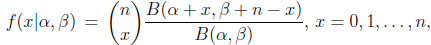
The univariate beta binomial model allows for extra binomial variation, i.e. overdispersion relative to the binomial model. It is constructed by taking a binomial model and assigning the binomial probability parameter p a beta distribution with parameters α and β. This model’s probability mass function is
 |
(1.1) |
where α > 0, β > 0, and B is the beta function. This beta binomial distribution is known by other names, including the negative hypergeometric distribution and the inverse hypergeometric distribution. A summary of the model’s development and early use is given in Johnson, Kotz, and Kemp [1N.L. Johnson, A.W. Kemp, and S. Kotz, Univariate Discrete Distributions., 3rd edJohn Wiley & Sons Inc.: New York, .
[http://dx.doi.org/10.1002/0471715816] ]. To cite a few examples, Skellam [2J.G. Skellam, "A probability distribution derived from the binomial distribution by regarding the probability of success as variable between the sets of trials", J. R. Stat. Soc. B, vol. 10, pp. 257-261.] applied the model to the association of chromosomes and to traffic clusters and Ishii and Hayakawa [3G. Ishii, and R. Hayakawa, "On the compound binomial distribution", Annals of the Institute of Statistical Mathematics, Tokyo, vol. 12, pp. 69-80.
[http://dx.doi.org/10.1007/BF01577666] ] used it as a model for the sex composition of families and for the absence of students.
Models that recognise overdispersion in the case of correlated bivariate count data are also naturally useful. The alternative of failing to recognise such overdispersion may lead to faulty statistical inferences and inaccurate conclusions due to an underestimation of the variability of the data. Some examples in the literature involving correlated overdispersed bivariate count data are Bibby and Væth [4B.M. Bibby, and M. Væth, "The two-dimensional beta binomial distribution", Stat. Probab. Lett., vol. 81, pp. 884-891.
[http://dx.doi.org/10.1016/j.spl.2010.12.019] ], who examined counts of diseased second premolars and second molars in Danish children’s upper jaws, and Danahar and Hardie [5P.J. Danaher, and B.G. Hardie, "Bacon with your eggs? Applications of a new bivariate beta-binomial distribution", Am. Stat., vol. 59, no. 4, pp. 282-286.
[http://dx.doi.org/10.1198/000313005X70939] ], who examined the number of bacon and eggs purchases made by households and also the joint readership of two magazines.
Bibby and Væth [4B.M. Bibby, and M. Væth, "The two-dimensional beta binomial distribution", Stat. Probab. Lett., vol. 81, pp. 884-891.
[http://dx.doi.org/10.1016/j.spl.2010.12.019] ] developed a two-dimensional beta binomial distribution based on the two-dimensional beta distribution introduced in Jones [6M. Jones, "Multivariate t and beta distributions associated with the multivariate t dis- tribution", Metrika, vol. 54, pp. 215-231.
[http://dx.doi.org/10.1007/s184-002-8365-4] ], using a construction similar to that in Skellam [2J.G. Skellam, "A probability distribution derived from the binomial distribution by regarding the probability of success as variable between the sets of trials", J. R. Stat. Soc. B, vol. 10, pp. 257-261.] for the one-dimensional case. Properties of this distribution were given and its estimation and computational aspects were also discussed. A number of additional two-dimensional beta binomial models were also presented. However, these additional models did not have closed forms of probability mass functions and thus were not amenable to analysis using maximum likelihood. This limited their applicability. Such as, they were not considered in detail nor were they applied to any data.
In this paper, we will consider the Bayesian analysis of all three models appearing in Bibby and Væth [4B.M. Bibby, and M. Væth, "The two-dimensional beta binomial distribution", Stat. Probab. Lett., vol. 81, pp. 884-891.
[http://dx.doi.org/10.1016/j.spl.2010.12.019] ], including the two with intractable forms. These models will be applied to a real data set describing student performances on tests in two related university courses. In Sections 2 and 3, the models under consideration will be presented. In Section 4, we discuss how a Bayesian analysis for any of these models may proceed on the basis of a Markov chain Monte Carlo (MCMC) set-up using data augmentation. The real data set will be analyzed in Section 5, where various approaches to model selection including the use of predictive information criteria will also be illustrated. OpenBUGS code associated with the numerical example appears in the Appendix.
2. THE TWO-DIMENSIONAL BETA BINOMIAL MODEL
Jones [6M. Jones, "Multivariate t and beta distributions associated with the multivariate t dis- tribution", Metrika, vol. 54, pp. 215-231.
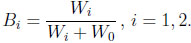
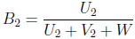
[http://dx.doi.org/10.1007/s184-002-8365-4] ] introduced the two-dimensional beta distribution described below. Let W0 , W1, and W2 be mutually independent random variables such that Wi χ2(2νi), i.e. Γ(νi, 1), for νi > 0. Now define
 |
(2.2) |
Then the resulting Bi is Beta(νi, ν0 )-distributed, for i = 1, 2. The two-dimensional beta distribution describes the joint distribution of B1 and B2, and its probability density function is given by Γ(ν)
 |
(2.3) |
for 0 < b1< 1, 0 < b2< 1, and ν = ν1 + ν2 + ν0 .
Bibby and Væth [1N.L. Johnson, A.W. Kemp, and S. Kotz, Univariate Discrete Distributions., 3rd edJohn Wiley & Sons Inc.: New York, .
[http://dx.doi.org/10.1002/0471715816] ] developed a two-dimensional beta binomial distribution in terms of the two-dimensional beta distribution in a manner analogous to the one dimensional case.
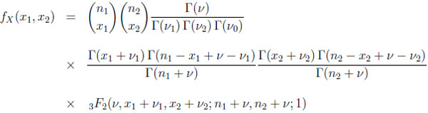
Let p = (p1, p2) be a two-dimensional beta random variable with parameters ν1, ν2, and ν0 . Given p, let X1 and X2 be two independent binomially distributed random variables, with Xi| p bin(ni, pi) for i = 1, 2. Then the joint distribution of X = (X1, X2) is known as the two-dimensional beta binomial distribution and its probability mass function is given by
 |
(2.4) |
for x1 = 0, 1, . . ., n1 and x2 = 0, 1, . . ., n2. This bivariate distribution will be denoted as
 |
(2.5) |
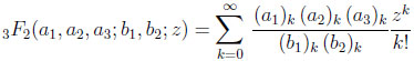
The form of the probability mass function given above in (2.4) is significantly complicated by the presence of a generalized hypergeometric function, denoted by 3F2 . The definition of this generalized hypergeometric function is given by
 |
(2.6) |
where the (a)k are the Pochhammer symbols
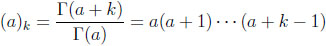 |
with (a)0 = 1. The series in (2.6) is convergent at the point z = 1 if and only if b1 + b2> a1 + a2 + a3. This convergence condition is always met in the context of the probability mass function in (2.4). See Bailey [7W.N. Bailey, "Generalized Hypergeometric Series", Cambridge Tracts in Mathematics and Mathematical Physics, vol. 32, Cambridge University Press, .] for additional details. Bibby and Væth [4B.M. Bibby, and M. Væth, "The two-dimensional beta binomial distribution", Stat. Probab. Lett., vol. 81, pp. 884-891.
[http://dx.doi.org/10.1016/j.spl.2010.12.019] ] observed that the calculation of the generalized hypergeometric function at the argument 1 is numerically unstable. This presents some problems when estimating the parameters of the two-dimensional beta binomial model using maximum likelihood. The Bayesian method presented later in this paper does not suffer from the same problems, as it circumvents the calculation of the generalized hypergeometric function entirely.
The two-dimensional beta binomial distribution is such that its marginal distributions are univariate beta binomial, that is
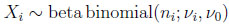 |
(2.7) |
for i = 1, 2. The marginal mean and variance are given by
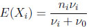 |
(2.8) |
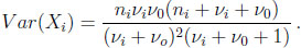 |
(2.9) |
From Bibby and Væth [1N.L. Johnson, A.W. Kemp, and S. Kotz, Univariate Discrete Distributions., 3rd edJohn Wiley & Sons Inc.: New York, .
[http://dx.doi.org/10.1002/0471715816] ], the correlation between the two marginals is given by
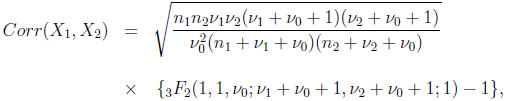 |
(2.10) |
and this correlation is always positive with a strictly positive lower bound, that is
 |
(2.11) |
3. TWO ADDITIONAL TWO-DIMENSIONAL BETA BINOMIAL MODELS
Several other two-dimensional beta binomial distributions were briefly considered in Bibby and Væth [4B.M. Bibby, and M. Væth, "The two-dimensional beta binomial distribution", Stat. Probab. Lett., vol. 81, pp. 884-891.
[http://dx.doi.org/10.1016/j.spl.2010.12.019] ], two of which are of interest here and will be reviewed below. Whereas the two- dimensional beta binomial distribution of the last section has a positive correlation between the marginals that is positive and bounded away from zero, the models introduced in this section include independent beta binomial marginal distributions as special cases.
The second two-dimensional beta binomial model replaces B1 and B2 in (2.2) with
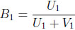 |
(3.12) |
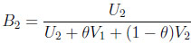 |
(3.13) |
where Ui Γ(νi, 1) and Vi Γ(ν0 , 1), for i = 1, 2, are all mutually independent. Let p = (p1, p2) be a two-dimensional random variable defined in accordance with (3.12) and (3.13). Given p, let X1 and X2 be two independent binomially distributed random variables as before, with Xi| p bin(ni, pi) for i = 1, 2. Then the resulting model for the joint distribution of X = (X1, X2) includes the two-dimensional beta binomial distribution (2.5) as a special case when θ = 1, and two independent univariate beta binomial distributions as another when θ = 0. As yet, there appears to be no closed form expression available for this model’s probability mass function and it may be that one does not exist.
The third of the two-dimensional beta binomial models uses
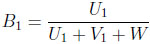 |
(3.14) |
 |
(3.15) |
where Ui Γ(µi, 1) and Vi Γ(νi, 1), for i = 1, 2, W Γ(ω, 1), and Ui, Vi, and W are all mutually independent. In this case, the resulting Bi random variables are Beta(µi, νi + ω)- distributed, for i = 1, 2. Let p = (p1, p2) be defined in accordance with (3.14) and (3.15) and let Xi| p bin(ni, pi), for i = 1, 2. Then the resulting model for the joint distribution of X = (X1, X2) includes the product of two independent beta binomial distributions as a limiting case when ω → 0. However, the joint density of B1 and B2 involves an integral of a product of two confluent hypergeometric functions leading to an intractable joint probability mass function for (X1, X2). Note, the third model’s construction bears some similarity to that of the previous two models and so it might casually be described as an extension of the first or second models. However, technically speaking the first and second models are not special cases of (i.e. are not nested within) the third.
As noted, the second and third models were introduced and briefly discussed in Bibby and Væth [4B.M. Bibby, and M. Væth, "The two-dimensional beta binomial distribution", Stat. Probab. Lett., vol. 81, pp. 884-891.
[http://dx.doi.org/10.1016/j.spl.2010.12.019] ]. However, neither model was used in the context of a numerical illustration. Indeed, these additional models do not have closed forms of probability mass functions and are not amenable to analysis using maximum likelihood. However, the Bayesian estimation method presented in the next section for the two-dimensional beta binomial distribution can be easily modified and applied.
4. BAYESIAN ESTIMATION VIA MCMC AND DATA AUGMENTATION
Estimation of the parameters appearing in the two-dimensional beta binomial model (2.5) using maximum likelihood is complicated by the presence of the generalized hypergeometric function in that model’s probability mass function. The additional two models presented in the last section pose even greater challenges for this estimation method. A Bayesian estimation method using MCMC and data augmentation can circumvent these challenges.
Consider a random sample of size N from a two-dimensional beta binomial distribution. Denote this sample as X = (X1, X2, . . ., XN ), where Xi = (Xi1, Xi2) is distributed according to the distribution in (2.4). The probability model
 |
(4.16) |
for i = 1, . . ., N and j = 1, 2, can be represented with the use of latent variables P and W as
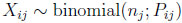 |
(4.17) |
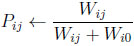 |
(4.18) |
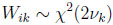 |
(4.19) |
for i = 1, . . ., N, j = 1, 2, and k = 0, 1, 2, in accordance with the development presented in Section 2.
It remains to assign a prior density specification to the unknown parameters νk , k = 0, 1, 2, and then implement a MCMC analysis (given the observed data) of the resulting full probability model based on (4.17) to (4.19). This may be accomplished with the assistance of any of a number of statistical computing packages presently available to implement Gibbs sampling or other more advanced forms of MCMC. For example in this paper, the OpenBUGS package was used. The OpenBUGS package is available at www.openbugs.net.
Illustrative OpenBUGS code corresponding to the example appearing in the next section is provided in the Appendix. With suitable elementary adjustments to the code, the two additional models presented in Section 3 can be analyzed in a likely manner. Some of the foundational papers on Gibbs sampling include Geman and Geman [8S. Geman, and D. Geman, "Stochastic relaxation, gibbs distributions, and the bayesian restoration of images", IEEE Trans. Pattern Anal. Mach. Intell., vol. 6, no. 6, pp. 721-741.
[http://dx.doi.org/10.1109/TPAMI.1984.4767596] [PMID: 22499653] ] and Gelfand and Smith [9A.E. Gelfand, and A.F. Smith, "Sampling-based approaches to calculating marginal densities", J. Am. Stat. Assoc., vol. 85, no. 410, pp. 398-409.
[http://dx.doi.org/10.1080/01621459.1990.10476213] ]. Any readers requiring information on how to implement, monitor, and analyse the results of a MCMC simulation are directed to Congdon [10P. Congdon, Bayesian Statistical Modelling., 2nd edJohn Wiley & Sons Ltd: West Sussex, .
[http://dx.doi.org/10.1002/9780470035948] ], Gelman et al. [11A. Gelman, J.B. Carlin, H.S. Stern, D.B. Dunson, A. Vehtari, D.B. Rubin, Bayesian Data Analysis., 3rd edChapman & Hall / CRC: New York, .], and the user manual that accompanies (i.e. accessible within) OpenBUGS. Manuals and additional resources are also available at www.openbugs.net/w/Documentation.
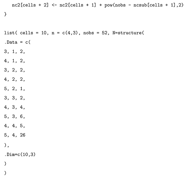
5. EXAMPLE
This example concerns the number of tests passed by 52 students in each of two distinct but related actuarial science courses at the University of Calgary in the same academic year. The two courses had the same prerequisites and the same instructor. We have applied the three models discussed in this paper to the data. The data are provided in Table 1.
For each model, a Bayesian method of analysis was adopted and implemented as described in the preceding section. The analysis for each model was performed separately and independent prior densities were assigned to each unknown (top-level) model parameter. Each of the model parameters νi, µi, and ω appearing in any given model was assigned an exponential prior distribution with a common mean of 10. This prior assigns a little over 63.2% and 86.4% of its mass to values below 10 and 20, respectively, and treats an interval of smaller values as being more probable than an interval of larger values with the same interval width, a priori. Although this prior is not noninformative, it is relatively diffuse over a large range of parameter values (e.g., values less than 20) containing what we consider to be a reasonable and a priori probable subrange (e.g., values less than 10). The parameter θ appearing in the first extended model was assigned a uniform prior on the interval (0, 1). For the problem under consideration the overall choice of prior density specification described above seemed reasonable. However, some other prior density specifications were also tried in conjunction with these models. Although the resulting posterior inferences changed slightly, the relative ranking of the models in terms of their fits and predictive performances (as discussed below) was essentially unchanged.
The MCMC based analysis in OpenBUGS used 4 chains, each was burned for 150,000 iterations, and then allowed to run for an additional 100,000 thus yielding 400,000 kept iterations. Tables 2 to 4 report the posterior means, standard deviations, 95% (symmetric) posterior density intervals, and 95% highest (i.e. shortest) posterior density (HPD) intervals for the top-level model parameters assuming the prior density specification mentioned earlier. These posterior summaries are primarily reported for completeness, and the values of the summaries in one table (e.g. for ν1 and ν2) are not meant to be compared to those in another. We note that the estimated posterior densities were all unimodal and skewed to varying degrees. The skewness is revealed by comparing a parameter’s symmetric posterior density interval to its HPD interval. If a parameter’s posterior density was symmetric and unimodal, these two intervals would be the same.

Recall that the data set contains 52 observations. As part of the MCMC based analysis, a predictive replicated sample of size 52 was generated from the model at each iteration. Summaries of these predictive replicated samples are reported in Tables 5 to 7. Specifically, these tables report the estimated predicted expected value and standard deviation of the number of students (assuming a cohort size of 52 students) in each combination of the number of tests passed in the two related actuarial science courses, under each model. One may observe that each model’s predicted row and column totals are (for the most part) generally in agreement with those for the original data in Table 1.
Table 5.

Table 8 summarizes the means and standard deviations of the number of tests passed in each course, along with the correlation between the two. The first rows of numerical values in this table are the empirical values associated with the observed data. These are followed by the Bayesian predictive values associated with the three models under consideration. In this example, it appears that while all three models generally replicate the empirical means and standard deviations, the first model does a much better job at replicating the correlation than either the second or third.
The means and standard deviations of the number of tests passed in each of the two courses, along with the correlation between the two courses. The first line gives the observed values corresponding to Table 1; the estimated predictive values associated with the first, second, and third models follow.
When the goal is to pick a model with the best out-of-sample predictive power then selection can be made on the basis of the deviance information criterion (DIC), which is a combined measure of goodness of fit and model complexity. The DIC and its calculation are discussed in Spiegelhalter et al. [12D.J. Spiegelhalter, N.G. Best, B.P. Carlin, and A. van der Linde, "Bayesian measures of model complexity and fit (with discussion)", J. R. Stat. Soc. B, vol. 64, pp. 583-640.
[http://dx.doi.org/10.1111/1467-9868.00353] ]. See also Chapter 7 in Gelman et al. [11A. Gelman, J.B. Carlin, H.S. Stern, D.B. Dunson, A. Vehtari, D.B. Rubin, Bayesian Data Analysis., 3rd edChapman & Hall / CRC: New York, .]. The DIC is implemented in OpenBUGS and according to the OpenBUGS User Manual, “the model with the smallest DIC is estimated to be the model that would best predict a replicate dataset of the same structure as that currently observed”. The values of the DIC corresponding to the models represented in Tables 5 to 7 are 162.9, 164.7, and 169.1, respectively. So based on this criterion, the first of the three models under consideration is the preferred model.
Although the DIC is conveniently incorporated in OpenBUGS, it is not without its problems. For instance, it can produce negative estimates of the effective number of parameters in its evaluation of a model’s complexity and it is not defined for singular models. See Celeux et al. [13G. Celeux, F. Forbes, C. Robert, and D. Titterington, "Deviance information criteria for missing data models", Bayesian Anal., vol. 1, pp. 651-706.
[http://dx.doi.org/10.1214/06-BA122] ], Gelman et al. [14A. Gelman, J. Hwang, and A. Vehtari, "Understanding predictive information criteria for Bayesian models", Stat. Comput., vol. 24, pp. 997-1016.
[http://dx.doi.org/10.1007/s11222-013-9416-2] ], Plummer [15M. Plummer, "Penalized loss functions for Bayesian model comparison", Biostatistics, vol. 9, no. 3, pp. 523-539.
[http://dx.doi.org/10.1093/biostatistics/kxm049] [PMID: 18209015] ], and Spiegelhalter et al. [16D.J. Spiegelhalter, N.G. Best, B.P. Carlin, and A. van der Linde, "The deviance information criterion: 12 years on", J. R. Stat. Soc. B, vol. 76, pp. 485-493.
[http://dx.doi.org/10.1111/rssb.12062] ]. The WAIC (Watanabe- Akaike or widely applicable information criterion; Watanabe [17S. Watanabe, "Asymptotic equivalence of Bayes cross validation and widely applicable information criterion in singular learning theory", J. Mach. Learn. Res., vol. 11, pp. 3571-3591.]) is another measure of a model’s predictive accuracy. This criterion is fully Bayesian and works for singular models and may be viewed as an improvement on the DIC (however, the WAIC is not without its own difficulties; see Gelman et al. [14A. Gelman, J. Hwang, and A. Vehtari, "Understanding predictive information criteria for Bayesian models", Stat. Comput., vol. 24, pp. 997-1016.
[http://dx.doi.org/10.1007/s11222-013-9416-2] ]). Unfortunately, the WAIC is not directly calculated by OpenBUGS, but it is not too difficult to evaluate it using output from OpenBUGS. We did so, using the definition for the version of WAIC found in Gelman et al. [14A. Gelman, J. Hwang, and A. Vehtari, "Understanding predictive information criteria for Bayesian models", Stat. Comput., vol. 24, pp. 997-1016.
[http://dx.doi.org/10.1007/s11222-013-9416-2] ] The values of the WAIC corresponding to the models represented in Tables 5 to 7 are 173.5, 177.4, and 185.7, respectively. Therefore, of the models under consideration, the first again exhibits the best predictive accuracy for the data in Table 1, this time according to the WAIC. We note that other predictive information criteria for Bayesian models do exist, several of which are reviewed by Gelman et al. [14A. Gelman, J. Hwang, and A. Vehtari, "Understanding predictive information criteria for Bayesian models", Stat. Comput., vol. 24, pp. 997-1016.
[http://dx.doi.org/10.1007/s11222-013-9416-2] ].
Another approach to checking model fit involves focusing attention on a particular test quantity or discrepancy measure of interest. This test quantity may be a function of the known and unknown parameters as well as of the data. Let such a test quantity be denoted as T (D, φ), with D denoting the data and φ the model parameters. If D pred denotes a predicted replicated data set generated from the model, then the predictive Bayesian p-value is defined as
 |
(5.20) |
where the probability is taken over the posterior distribution of φ and the posterior predictive distribution of D pred. Extreme values of T (D pred, φ) relative to T (D, φ) are evidence of discrepancy between the model and the data. Thus, a Bayesian p-value near 0 or 1 provides evidence of model discrepancy. See Gelman et al. [11A. Gelman, J.B. Carlin, H.S. Stern, D.B. Dunson, A. Vehtari, D.B. Rubin, Bayesian Data Analysis., 3rd edChapman & Hall / CRC: New York, .] for a more detailed discussion of Bayesian p-values.
In the present context of an example involving correlated bivariate data, a sensible and meaningful discrepancy measure is the sample correlation. In the original data set, the sample correlation r = T (D, φ) is equal to 0.667. Recall, as part of our MCMC based analysis, a predictive replicated sample of size 52 was generated from the model under study at each iteration. For each model, we monitored the posterior predictive distribution of the sample correlation for the replicated data, i.e.r pred = T (D pred, φ), and monitored its relation to the sample correlation of the original data. The results are presented in Table 9, and lend further support to the conclusion that the first of the three models under consideration is a better fit to the data than either of the two extended models.
One final check of predictive model performance was performed. For each predictive replicated sample, the sum of squared deviations between the predicted and observed cell counts was calculated over the original non-empty cells. Denote this statistic as SS pred. When comparing models, smaller values of this statistic are indicative of a better fit. The estimated posterior predictive summaries for SS pred are reported in Table 10. Once again, the first of the three models under consideration comes out on top.
CONCLUSION
This paper considered three two-dimensional beta binomial models. Two of these models do not have closed forms of probability mass functions and are not amenable to analysis using maximum likelihood. Instead, a Bayesian analysis of each model was implemented using MCMC with data augmentation.
In the example contained within this paper, the first of the two-dimensional beta binomial models was the best performing model of the three considered. Of course, this does not necessarily mean that it will always perform better than the other two. However, as yet we have not run across an actual data set for which the first model did not perform at least as well as one of the others.
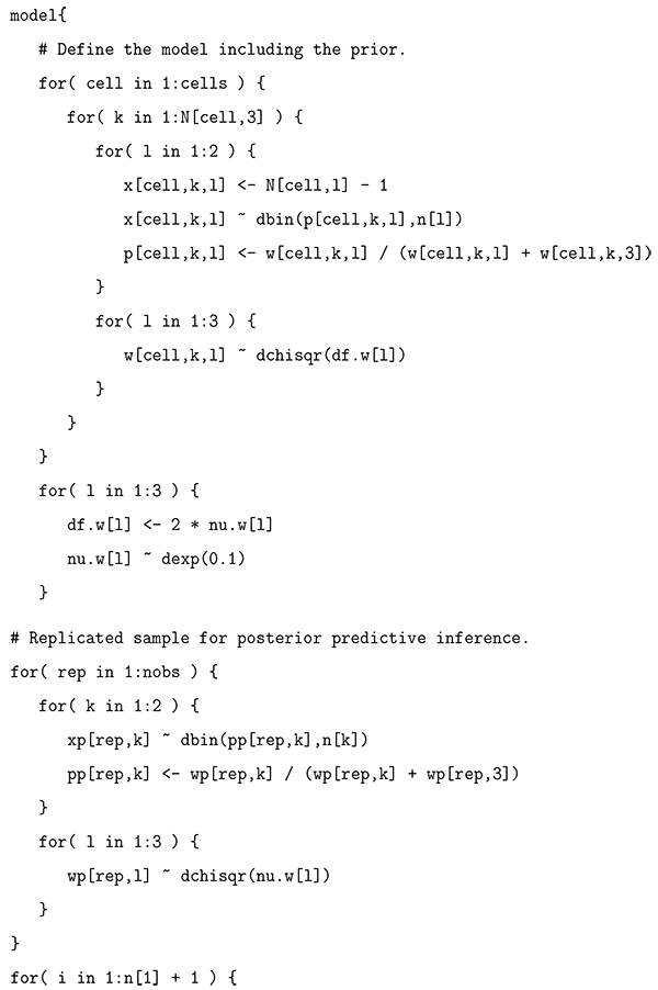
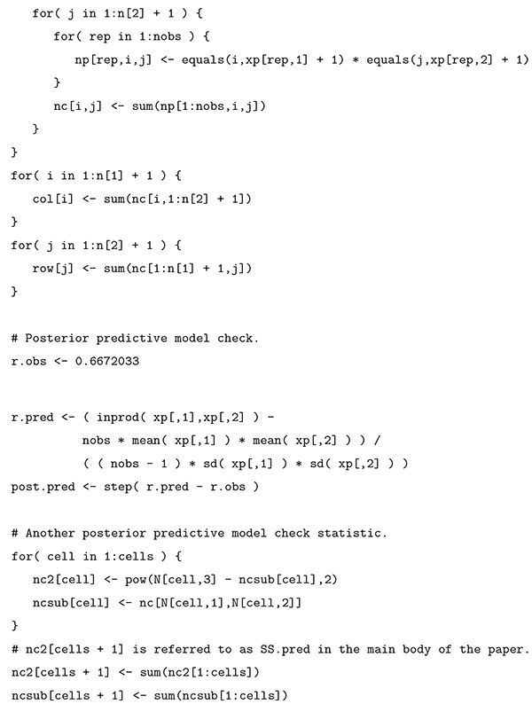
APPENDIX
This BUGS code can be used with OpenBUGS to implement a Bayesian analysis of the two- dimensional beta binomial model presented in Bibby and Væth [4B.M. Bibby, and M. Væth, "The two-dimensional beta binomial distribution", Stat. Probab. Lett., vol. 81, pp. 884-891.
[http://dx.doi.org/10.1016/j.spl.2010.12.019] ]. The manner of variable indexing and data formatting used in this code is such that tables containing cells with zero counts may be conveniently analysed. Only cells with non-zero counts are read in as data.
CONSENT FOR PUBLICATION
Not applicable.
CONFLICT OF INTEREST
The author declares no conflict of interest, financial or otherwise.
ACKNOWLEDGEMENTS
This research was supported by a Discovery Grant from the Natural Sciences and Engineering Research Council of Canada (NSERC).
REFERENCES
| [1] | N.L. Johnson, A.W. Kemp, and S. Kotz, Univariate Discrete Distributions., 3rd edJohn Wiley & Sons Inc.: New York, . [http://dx.doi.org/10.1002/0471715816] |
| [2] | J.G. Skellam, "A probability distribution derived from the binomial distribution by regarding the probability of success as variable between the sets of trials", J. R. Stat. Soc. B, vol. 10, pp. 257-261. |
| [3] | G. Ishii, and R. Hayakawa, "On the compound binomial distribution", Annals of the Institute of Statistical Mathematics, Tokyo, vol. 12, pp. 69-80. [http://dx.doi.org/10.1007/BF01577666] |
| [4] | B.M. Bibby, and M. Væth, "The two-dimensional beta binomial distribution", Stat. Probab. Lett., vol. 81, pp. 884-891. [http://dx.doi.org/10.1016/j.spl.2010.12.019] |
| [5] | P.J. Danaher, and B.G. Hardie, "Bacon with your eggs? Applications of a new bivariate beta-binomial distribution", Am. Stat., vol. 59, no. 4, pp. 282-286. [http://dx.doi.org/10.1198/000313005X70939] |
| [6] | M. Jones, "Multivariate t and beta distributions associated with the multivariate t dis- tribution", Metrika, vol. 54, pp. 215-231. [http://dx.doi.org/10.1007/s184-002-8365-4] |
| [7] | W.N. Bailey, "Generalized Hypergeometric Series", Cambridge Tracts in Mathematics and Mathematical Physics, vol. 32, Cambridge University Press, . |
| [8] | S. Geman, and D. Geman, "Stochastic relaxation, gibbs distributions, and the bayesian restoration of images", IEEE Trans. Pattern Anal. Mach. Intell., vol. 6, no. 6, pp. 721-741. [http://dx.doi.org/10.1109/TPAMI.1984.4767596] [PMID: 22499653] |
| [9] | A.E. Gelfand, and A.F. Smith, "Sampling-based approaches to calculating marginal densities", J. Am. Stat. Assoc., vol. 85, no. 410, pp. 398-409. [http://dx.doi.org/10.1080/01621459.1990.10476213] |
| [10] | P. Congdon, Bayesian Statistical Modelling., 2nd edJohn Wiley & Sons Ltd: West Sussex, . [http://dx.doi.org/10.1002/9780470035948] |
| [11] | A. Gelman, J.B. Carlin, H.S. Stern, D.B. Dunson, A. Vehtari, D.B. Rubin, Bayesian Data Analysis., 3rd edChapman & Hall / CRC: New York, . |
| [12] | D.J. Spiegelhalter, N.G. Best, B.P. Carlin, and A. van der Linde, "Bayesian measures of model complexity and fit (with discussion)", J. R. Stat. Soc. B, vol. 64, pp. 583-640. [http://dx.doi.org/10.1111/1467-9868.00353] |
| [13] | G. Celeux, F. Forbes, C. Robert, and D. Titterington, "Deviance information criteria for missing data models", Bayesian Anal., vol. 1, pp. 651-706. [http://dx.doi.org/10.1214/06-BA122] |
| [14] | A. Gelman, J. Hwang, and A. Vehtari, "Understanding predictive information criteria for Bayesian models", Stat. Comput., vol. 24, pp. 997-1016. [http://dx.doi.org/10.1007/s11222-013-9416-2] |
| [15] | M. Plummer, "Penalized loss functions for Bayesian model comparison", Biostatistics, vol. 9, no. 3, pp. 523-539. [http://dx.doi.org/10.1093/biostatistics/kxm049] [PMID: 18209015] |
| [16] | D.J. Spiegelhalter, N.G. Best, B.P. Carlin, and A. van der Linde, "The deviance information criterion: 12 years on", J. R. Stat. Soc. B, vol. 76, pp. 485-493. [http://dx.doi.org/10.1111/rssb.12062] |
| [17] | S. Watanabe, "Asymptotic equivalence of Bayes cross validation and widely applicable information criterion in singular learning theory", J. Mach. Learn. Res., vol. 11, pp. 3571-3591. |