- Home
- About Journals
-
Information for Authors/ReviewersEditorial Policies
Publication Fee
Publication Cycle - Process Flowchart
Online Manuscript Submission and Tracking System
Publishing Ethics and Rectitude
Authorship
Author Benefits
Reviewer Guidelines
Guest Editor Guidelines
Peer Review Workflow
Quick Track Option
Copyediting Services
Bentham Open Membership
Bentham Open Advisory Board
Archiving Policies
Fabricating and Stating False Information
Post Publication Discussions and Corrections
Editorial Management
Advertise With Us
Funding Agencies
Rate List
Kudos
General FAQs
Special Fee Waivers and Discounts
- Contact
- Help
- About Us
- Search


The Open Atmospheric Science Journal
(Discontinued)
ISSN: 1874-2823 ― Volume 14, 2020
Capturing Day-to-day Diurnal Variations in Stability in the Convective Atmospheric Boundary Layer Using Large Eddy Simulation
Jordan Nielson, Kiran Bhaganagar*
Abstract
Introduction:
Large Eddy Simulation (LES) modelers must begin to answer the question of how to better incorporate large datasets into simulations. This question is important because, at a given location, the diurnal, seasonal, and day-to-day variations of atmospheric stability have significant consequences for the power generated by wind turbines. The following study provides a methodology to obtain discrete values of surface flux, inversion height and geostrophic wind for LES using field data over multiple diurnal cycles (averaged over a month) at 12 Local Time (LT) (during the convective ABL). The methodology will allow the discrete LES to quantify the day-to-day variations over multiple diurnal cycles.
Methods:
The study tests the hypothesis that LES can capture the mean velocity and TKE profiles from the averaged variations in surface heat flux at 12 LT measured in the field (mean, +1 standard deviation, and -1 standard deviation). The discrete LES from the mean, +1 standard deviation, and -1 standard deviation surface heat flux represent the variations in the ABL due to the day-to-day variations in surface heat flux. The method calculates the surface heat flux for the NREL NWTC M5 dataset. The field data were used to generate Probability Density Functions (PDFs) of surface heat flux for the January and July 12 LT. The PDFs are used to select the surface heat fluxes as inputs into the discrete LES.
Results / Conclusion:
A correlation function between the surface heat flux and the boundary layer height was determined to select the initial inversion height, and the geostrophic departure function was used to determine the geostrophic wind for each surface heat flux. The LES profiles matched the averaged velocity profiles from the field data to 4% and the averaged TKE profiles to 6% and, therefore, validated the methodology. The method allows for further quantification of day-to-day stability variations using LES.
Article Information

Identifiers and Pagination:
Year: 2018Volume: 12
First Page: 107
Last Page: 131
Publisher Id: TOASCJ-12-107
DOI: 10.2174/1874282301812010107
Article History:
Received Date: 28/7/2018Revision Received Date: 22/10/2018
Acceptance Date: 10/11/2018
Electronic publication date: 30/11/2018
Collection year: 2018
open-access license: This is an open access article distributed under the terms of the Creative Commons Attribution 4.0 International Public License (CC-BY 4.0), a copy of which is available at: https://creativecommons.org/licenses/by/4.0/legalcode. This license permits unrestricted use, distribution, and reproduction in any medium, provided the original author and source are credited.
* Address correspondence to this author at Laboratory of Turbulence, Sensing and Intelligence Systems, Department of Mechanical Engineering, University of Texas, San Antonio, Texas, USA; Tel: +1-210-458-6497; E-mail: Kiran.bhaganagar@utsa.edu
| Open Peer Review Details | |||
|---|---|---|---|
| Manuscript submitted on 28-7-2018 |
Original Manuscript | Capturing Day-to-day Diurnal Variations in Stability in the Convective Atmospheric Boundary Layer Using Large Eddy Simulation | |
1. INTRODUCTION
Overland, the surface heat exchange between the ground and the atmosphere is an important driving mechanism for Atmospheric Boundary Layer (ABL) dynamics. The exchange results in a pronounced diurnal cycle in temperature, wind, depth and related ABL variables [1Carruthers DJ, Holroyd RJ, Hunt JCR, et al. UK-ADMS: A new approach to modelling dispersion in the earth’s atmospheric boundary layer. J Wind Eng Ind Aerodyn 1994; 52: 139-53.
[http://dx.doi.org/10.1016/0167-6105(94)90044-2] -3Stull RB. An introduction to boundary layer meteorology 2012; Vol. 13]. During the daytime conditions, the convective heat exchange between the surface and the atmosphere causes the large-scale buoyancy forcing from the surface that drives the ABL to be in a convective stability state. The surface heat exchange results in large-scale vertical motions that generate turbulence mainly dominated by the buoyancy-production mechanisms (and less from the shear-production) of Turbulence Kinetic Energy (TKE) resulting in a deeper ABL [3Stull RB. An introduction to boundary layer meteorology 2012; Vol. 13, 4Moeng C-H. A large-eddy-simulation model for the study of planetary boundary-layer turbulence. J Atmos Sci 1984; 41: 2052-62.
[http://dx.doi.org/10.1175/1520-0469(1984)041<2052:ALESMF>2.0.CO;2] ]. Higher turbulence results in a well-mixed layer within the convective ABL where the mean vertical gradients of wind velocity and potential temperature variables are nearly zero in this layer [5Johansson C, Smedman A-S, Högström U, Brasseur JG, Khanna S. Critical test of the validity of Monin–Obukhov similarity during convective conditions. J Atmos Sci 2001; 58: 1549-66.
[http://dx.doi.org/10.1175/1520-0469(2001)058<1549:CTOTVO>2.0.CO;2] , 6Carson DJ. The development of a dry inversion-capped convectively unstable boundary layer. Q J R Meteorol Soc 1973; 99: 450-67.
[http://dx.doi.org/10.1002/qj.49709942105] ]. An inversion layer at the top of the mixed layer caps the convective ABL. During nighttime conditions, the surface is colder than the atmosphere above, and the turbulence generated in the ABL is a balance between a positive TKE shear production and a negative buoyancy production [7Bhaganagar K, Debnath M. The effects of mean atmospheric forcings of the stable atmospheric boundary layer on wind turbine wake. J Renew Sustain Energy 2015; 7: 013124.
[http://dx.doi.org/10.1063/1.4907687] , 8Paulson CA. The mathematical representation of wind speed and temperature profiles in the unstable atmospheric surface layer. J Appl Meteorol 1970; 9: 857-61.
[http://dx.doi.org/10.1175/1520-0450(1970)009<0857:TMROWS>2.0.CO;2] ]. During nighttime conditions, the ABL is in a stable stability state characterized by a shallower layer with weak and intermittent turbulence.
Various field experiments [9Barr AG, Betts AK. Radiosonde boundary layer budgets above a boreal forest. J Geophys Res Atmos 1997; 102: 29205-12.
[http://dx.doi.org/10.1029/97JD01105] , 10Barr AG, Betts AK, Desjardins RL, MacPherson JI. Comparison of regional surface fluxes from boundary-layer budgets and aircraft measurements above boreal forest. J Geophys Res Atmos 1997; 102: 29213-8.
[http://dx.doi.org/10.1029/97JD01104] ] have confirmed that the vertical flux divergence (between the top flux and surface flux) plays a significant role in the time change of potential temperature in the ABL by analyzing the ABL budgets of sensible heat. In general, the top flux is a fraction of the surface flux; hence the ABL dynamics are dictated by the surface flux. These surface fluxes have significant variations. Grimmond and Oke [11Grimmond CSB, Oke TR. Comparison of heat fluxes from summertime observations in the suburbs of four North American cities. J Appl Meteorol 1995; 34: 873-89.
[http://dx.doi.org/10.1175/1520-0450(1995)034<0873:COHFFS>2.0.CO;2] ] compared summer heat fluxes at four different locations. They showed large day-to-day variations in the peak surface heat flux in all four areas. The most significant variations occurred around 12 Local Time (LT) for each of the four cities. The same is true for the variation in surface temperatures [12Yusuf N, Okoh D, Musa I, Adedoja S, Said R. A study of the surface air temperature variations in Nigeria. Open Atmos Sci J 2017; 11: 54-70.].
In Large Eddy Simulation (LES) of Atmospheric Boundary Layer (ABL) models, such as, SOWFA, the surface heat exchange processes are represented as surface heat flux and surface temperature specified as lower boundary conditions [4Moeng C-H. A large-eddy-simulation model for the study of planetary boundary-layer turbulence. J Atmos Sci 1984; 41: 2052-62.
[http://dx.doi.org/10.1175/1520-0469(1984)041<2052:ALESMF>2.0.CO;2] , 13Churchfield M J, Moriarty P J, Vijayakumar G, Brasseur J G. Wind Energy-Related Atmospheric Boundary-Layer Large-Eddy Simulation Using OpenFOAM. Natl. Renew Energy Lab Gold CO Rep. No NRELCP-500-48905 2010.-15Maldaner S, Degrazia AG, Rizza U. Derivation of the turbulent time scales and velocity variances from lES spectral data: Application in a lagrangian stochastic dispersion model. Open Atmos Sci J 2014; 8: 16-21.]. Overland, significant diurnal changes in the heat flux balance occur. Hence, the prediction of the ground surface temperature and surface heat flux is critical to obtain successful forecasts of the ABL dynamics. Most of the LES studies are idealistic and simulate quasi-steady ABL flows, as constant surface flux boundary conditions are imposed on the lower boundary. However, there is no consistent methodology to incorporate the surface flux measurements obtained from the field data. Obtaining these values is a challenging problem that stems from large day-to-day variations in surface heat flux measurements.
Recent advances in Large Eddy Simulation (LES) allowed researchers to perform a simulation of a diurnal cycle in the ABL [16Kumar V, Kleissl J, Meneveau C, Parlange MB. Large-eddy simulation of a diurnal cycle of the atmospheric boundary layer: Atmospheric stability and scaling issues. Water Resour Res 2006; 42: W06D09.
[http://dx.doi.org/10.1029/2005WR004651] -18Basu S, Vinuesa J-F, Swift A. Dynamic LES modeling of a diurnal cycle. J Appl Meteorol Climatol 2008; 47: 1156-74.
[http://dx.doi.org/10.1175/2007JAMC1677.1] ]. LES modelers achieve the diurnal cycle by changing the surface heat flux in real time. Kumar et al. [16Kumar V, Kleissl J, Meneveau C, Parlange MB. Large-eddy simulation of a diurnal cycle of the atmospheric boundary layer: Atmospheric stability and scaling issues. Water Resour Res 2006; 42: W06D09.
[http://dx.doi.org/10.1029/2005WR004651] ] used surface heat flux data from the HATS experiments to generate the surface heat flux boundary condition (over 24 hours) in LES. The simulation captured both convective and stable atmospheric conditions including the entrainment-based growth of the convective ABL, nocturnal jets, and mean velocity profiles.
The ability to perform LES of the diurnal cycle led to the study of wind turbines through a diurnal cycle. Lee and Lundquist [19Lee JC, Lundquist JK. Observing and simulating wind-turbine wakes during the evening transition 2017; 1-26.] studied the wake evolution during evening transition of the diurnal cycle using WRF. Their research showed that the wind farm created a 10% increase in wind-speed deficits, a 50% increase in TKE, and a 20% increase in surface heat flux during the convective ABL. Akbar et al. [20Abkar M, Sharifi A, Porté-Agel F. Wake flow in a wind farm during a diurnal cycle. J Turbul 2016; 17: 420-41.
[http://dx.doi.org/10.1080/14685248.2015.1127379] ] studied wake flow in a wind farm during the diurnal cycle and showed that increased mixing during the convective ABL reduces power deficits from 56% to 28%. The results confirm other studies that compared stable and convective wakes in wind farms [13Churchfield M J, Moriarty P J, Vijayakumar G, Brasseur J G. Wind Energy-Related Atmospheric Boundary-Layer Large-Eddy Simulation Using OpenFOAM. Natl. Renew Energy Lab Gold CO Rep. No NRELCP-500-48905 2010., 21Abkar M, Porté-Agel F. Influence of atmospheric stability on wind-turbine wakes: A large-eddy simulation study. Phys Fluids 2015; 27: 035104.
[http://dx.doi.org/10.1063/1.4913695] -23Chamorro LP, Porté-Agel F. A wind-tunnel investigation of wind-turbine wakes: Boundary-layer turbulence effects. Boundary-Layer Meteorol 2009; 132: 129-49.
[http://dx.doi.org/10.1007/s10546-009-9380-8] ].
These studies allow for the ability to look at variations in wind energy for a single diurnal cycle, but there are also variations that occur over multiple diurnal cycles. One outstanding question is how do the day-to-day variations in the strength of stability affect energy production in wind farms? The current study seeks to begin to answer this question by focusing on the day-to-day variations in surface heat flux because it is used in LES as a boundary condition to drive stability. The study tests the hypothesis that LES can capture the mean velocity and TKE profiles from the averaged variations in peak surface heat flux measured in the field (mean, +1 standard deviation, and -1 standard deviation). The study investigates the variations in multiple diurnal cycles by averaging the measured surface heat flux at each hour for an entire month. The focus is on the variations at 12 LT. The study tests the hypothesis using measured field data from the National Renewable Energy Laboratory (NREL) National Wind technology center (NWTC) M5 met tower in Colorado [24Clifton A, Schreck S, Scott G, Kelley N, Lundquist JK. Turbine inflow characterization at the national wind technology center. J Sol Energy Eng 2013; 135: 031017-031017-11.
[http://dx.doi.org/10.1115/1.4024068] , 25Clifton A. An unofficial guide to data products from the NWTC 135-m Meteorological Towers 2007.]. The methodology will aid in quantifying the effects of day-to-day variations of stability on wind energy production which will allow for an accounting of the variations in multiple diurnal cycles.
In this study, we will use the field data to determine the inputs of surface heat flux, inversion height, and geostrophic wind for the discrete LES of the ABL. The field data comes from a Meteorological tower that has wind, temperature, and pressure measurements at multiple heights (see Appendix A for a complete description) [24Clifton A, Schreck S, Scott G, Kelley N, Lundquist JK. Turbine inflow characterization at the national wind technology center. J Sol Energy Eng 2013; 135: 031017-031017-11.
[http://dx.doi.org/10.1115/1.4024068] , 25Clifton A. An unofficial guide to data products from the NWTC 135-m Meteorological Towers 2007.]. The tower is 135 m tall and, therefore, the geostrophic wind and inversion heights are not directly measured, but are determined using the wind speed and temperature measurements. Sonic anemometers allow for a direct measurement of turbulent fluctuations for both wind speed and temperature so that Turbulent Kinetic Energy (TKE) can be computed. The turbulent fluctuations for wind and temperature at 3 m are used to estimate the surface heat flux.
The objectives of the study are as follows:
- To understand the day-to-day variations of surface flux and its implications on the LES of wind turbines simulations
- To develop a methodology to obtain discrete values of surface flux, inversion height and geostrophic wind for LES that represent the day-to-day variations (of a given month)
- To select the best fit probability function for surface heat flux
- To understand the correlation between the variability in surface heat flux with turbulence kinetic energy, friction velocity, wind speed, and wind shear
- To validate the TKE and velocity profiles obtained from LES using the above boundary conditions with averaged field data over specified surface heat flux and wind speed of January and July 2016
The manuscript is as follows. The methodology for using the field data and setting up LES is described in Section 2. The results and discussion are shown in Section 3. The conclusions are presented in Section 4.
2. METHODOLOGY
2.1. Methodology and NREL NWTC Data
Fig. (1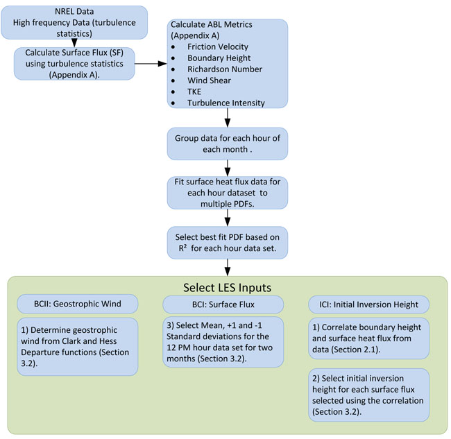 ) shows a brief overview of the methodology. The overall idea is to conduct discrete LES that represents day-to-day variations in atmospheric stability using realistic boundary conditions from field data. The LES tool requires discrete values for surface heat flux on the lower boundary, initial inversion height (specified using a 3-layer temperature profile as explained in section 2.2), and geostrophic wind on the upper boundary. The methodology consists of following steps, which will be explained in detail in this section: (1) Obtaining the instantaneous surface heat flux from the field data, (2) gathering the surface heat flux data occurring between 12-13 LT (for each month), (3) fitting the gathered data to multiple Probability Density Functions (PDFs), (4) selecting the best fit PDF using, and (5) determining the discrete boundary conditions required for LES using the surface heat flux PDF. The inversion height for each surface heat flux is determined from the field data correlation between surface heat flux and boundary height as shown in Fig. (5
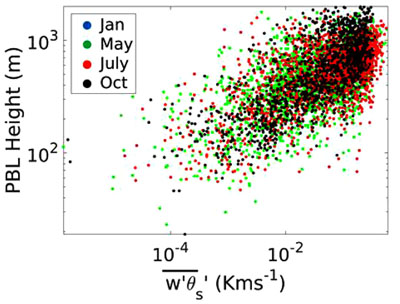 ). The geostrophic wind for each surface heat flux is determined from the departure function defined by Clarke and Hess [26Clarke RH, Hess GD. Geostrophic departure and the functions A and B of Rossby-number similarity theory. Boundary-Layer Meteorol 1974; 7: 267-87.
[http://dx.doi.org/10.1007/BF00240832] ].
The PDF for the data occurring between 12LT-13LT represents the day-to-day variations at 12LT for an entire month. The study uses the PDF to determine discrete values for the surface heat flux data occurring between 12LT-13LT. The discrete surface heat flux values become inputs into LES in addition to the corresponding initial inversion height, and geostrophic wind. The LES profiles are compared to the field data wind speed and TKE profiles to validate the methodology. The Correlations of surface heat flux and: TKE, friction velocity, wind shear, and wind speed for the LES simulations and measured data are compared to understand the implications of day-to-day variations on wind turbines.
The data used in this study is from the 135-m tall M5 meteorological tower installed at the NREL NWTC near Boulder Colorado [27 NWTC Information Portal (NWTC 135-m Meteorological Towers Data Repository).
https:// nwtc.nrel.gov/ 135mData Last modified 01-April-2015 ; Accessed 21-October-2018.]. The data consists of high-frequency measurements of wind speed, wind direction and air temperature at elevations of 15, 30, 50, 76, 100, and 131 above the ground January, May, July and October of the year 2016. These months correspond to Winter, Spring, Summer, and Fall for that year. For our analysis, the measured data were used to obtain the derived atmospheric variables, namely, Surface heat flux, atmospheric boundary layer height, wind shear, and Turbulent Kinetic Energy (TKE) (see Appendix A for details [24Clifton A, Schreck S, Scott G, Kelley N, Lundquist JK. Turbine inflow characterization at the national wind technology center. J Sol Energy Eng 2013; 135: 031017-031017-11.
[http://dx.doi.org/10.1115/1.4024068] ].
Fig. (2a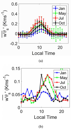 ) shows the monthly-averaged surface heat flux for each hour of the day for January, May, July, and October. The vertical bars denote one standard deviation (+1σ to -1σ) from the mean. Fig. (2b) shows the standard deviation (σ) of the surface heat flux at each hour. In general, a positive value of surface heat flux refers to convective stability state of the atmosphere, whereas negative values denote a stable atmosphere, and a zero value refers to a neutral atmosphere [3Stull RB. An introduction to boundary layer meteorology 2012; Vol. 13]. The strength of the stability is related to the magnitude of the value. Significant differences in both the values of the mean surface flux and the standard deviation from the mean is observed between the 4 selected months. The mean surface heat flux during the early morning hours (00 to 05 LT) is negative for all the 4 months with values ranging from -0.0295 kms-1 for January to -0.158 kms-1 for May. Positive mean surface heat flux occurs between times of 9-15 LT, 6-16 LT, 6-17 LT, and 7-15 LT for January, May, July, and October respectively. The maximum mean surface heat flux occurs near 12 LT for all the months, but the magnitude ranges from 0.088, 0.234, 0.231, and 0.177 kms-1 for January, May, July, and October respectively. During the later hours, the mean surface heat flux transitions back to negative values.
 |
Fig. (1) Methodology to incorporate boundary and initial conditions into LES. |
 |
Fig. (2) Mean and variability of surface heat flux at different hours for different months using NREL data. (a) shows the mean and one standard deviation error bars (b) shows the standard deviation. |
Fig. (2b) shows the month of October to have the highest standard deviations from the mean at 10 LT with a standard deviation of 0.126 kms-1 whereas, for July, the highest standard deviation is 0.125 kms-1 at 12 LT. The highest standard deviation for January and May is 0.070 kms-1 and 0.124 kms-1 which occur at 10LT and 12LT respectively. The July 12 LT standard deviation is nearly 58% of the mean surface heat flux at that hour, which indicates the day-to-day variations of the surface flux are significant. It is interesting to observe that though the general trend of mean surface heat flux is similar for all the months; the standard deviation from the mean does not follow the same trend. The difference is due to the fact the maximum mean surface heat flux for the summer month of July is over two times the value than January. The difference in maximum mean surface heat flux occurs even though the minimum values of the mean surface heat flux are comparable between all the 4 months. July exhibits the highest peak surface flux, but the variability is highest for May, July, and May.
The magnitude and variation of surface heat flux changes between different seasons, especially during the convective portion of the day from 8 to 16 LT. July shows the largest mean surface heat flux of 0.24 kms-1 with its highest standard deviations of 0.125 kms-1 at 12 LT while January shows the lowest mean surface heat flux of 0.088 kms-1 and the lowest standard deviation of 0.06 kms-1 at 12 LT. The results show clear seasonal (differences between the four months) and diurnal variations in surface heat flux exist between these four months. In addition, the surface heat flux standard deviation from the mean shows a day-to-day variation as well.
The day-to-day variations over multiple diurnal cycles are studied. For this purpose, a scatter plot of 10-min averaged surface heat flux for the entire month at a given time is analyzed. Fig. (3a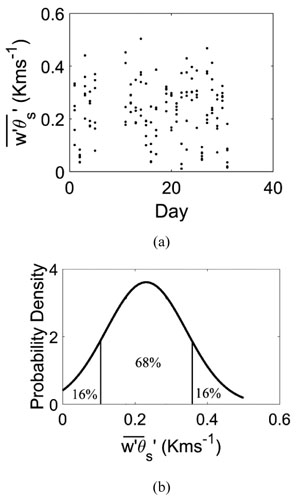 ) shows the 10-minute averaged surface heat flux for averaged data that falls between 12 LT and 13 LT time for all the days of July (referred to as July 12LT). The x-axis of is the day of the month for July 2016. The figure shows significant day-to-day variations in surface heat flux with the highest value of 0.52 kms-1 and the lowest value of 0.05 kms-1. The day-to-day variations observed in the average surface heat flux for the July 12 LT can be well represented using a Probability Density Function (PDF) using mathematical probability theory [28Hogg RV, Craig AT. Introduction to mathematical statistics(5th edition) 1995.]. A normal PDF fitted to the data from July 12 LT is shown in Fig. (3b). Fitted in this manner, 68% of the data is within the ±1σ, 95% of the data is within ±2σ, and 99% fall within ±3σ.
The PDF represents the variability at 12LT and will be used to select the inputs for LES. The actual PDF is determined in section 3.1. The focus of the current study is on day-to-day variations, particularly for the July 12 LT, because of the large mean surface heat flux and standard deviation from the mean that occurs at that time. In addition, the January 12 LT will also be studied to investigate the implications of smaller mean and standard deviation from the mean of the surface heat flux.
 |
Fig. (3) (a) 10 min averaged surface heat flux for the July 12 LT local time for each day (b) probability density function for the July 12 LT local time surface heat flux. |
Next, we investigate the correlations of the surface heat flux with TKE and ABL height. The correlation with TKE helps to understand how the variations in surface heat flux will impact the output of the LES. Fig. (4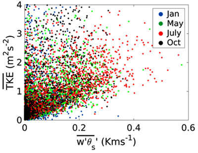 ) shows the correlation of 10-min averaged surface heat flux and TKE for different months of the NREL data at an elevation of 76 m above the ground. There is a positive correlation between surface heat flux and TKE (R2 of 0.45). The low R2 indicates some variability, but the correlation has a p-value <0.01 indicating the correlation is significant even with the variability. The methodology to incorporate surface heat flux variations into LES will need to capture the relationships shown to be used in LES applications. The surface heat flux correlations will be used to validate the LES in section 3.3.
 |
Fig. (4) Correlation of heat flux and TKE at 76 m during convective hours for different months. |
Finally, we investigate the correlation between surface heat flux and the approximated ABL height (shown in Eq. 16). The relationship is shown by plotting the two on a log-log scaled plot as seen in Fig. (5). The data show a positive correlation. The correlation function between surface heat flux and ABL height is a power law, described as  , rather than linear as found with TKE. This relationship had slightly less variability than TKE with an R2 value of 0.55 compared to 0.47. Again, the p-value is <0.01, which indicates significance to the correlation. The correlation function
  is used to obtain the initial inversion height for LES simulations based on the boundary condition given for surface heat flux [29Sugiyama G, Nasstrom JS. Methods for determining the height of the atmospheric boundary layer. Lawrence Livermore Natl. Lab Intern Rep UCRL-ID-133200 1999.].
 |
Fig. (5) Correlation of surface heat flux and ABL height during convective hours for different months. |
In summary, the NWTC Metrological tower data for January, May, October, and December 2016 shows the presence of day-to-day variability of surface heat flux over multiple diurnal cycles. Results have been shown for July 12 LT. However, all four months show similar trends (section 3.1). These results are comparable to Grimmond and Oke [11Grimmond CSB, Oke TR. Comparison of heat fluxes from summertime observations in the suburbs of four North American cities. J Appl Meteorol 1995; 34: 873-89.
[http://dx.doi.org/10.1175/1520-0450(1995)034<0873:COHFFS>2.0.CO;2] ] who showed the largest day-to-day variations of surface heat flux occur near midday. The 10-minute averaged surface heat flux showed correlations with both TKE and ABL height, which is also described by Obukhov theory [30Foken T. 50 years of the Monin–Obukhov similarity theory. Boundary-Layer Meteorol 2006; 119: 431-47.
[http://dx.doi.org/10.1007/s10546-006-9048-6] ]. A linear correlation exists between the averaged surface heat flux and TKE, whereas the correlation is a power law with the ABL height. The correlations have implications to the modeling of LES. The variations of surface heat flux affect the TKE output of the simulation, which is important in may LES applications. The study investigates multiple PDFs to best define the variations in surface heat flux. The study uses multiple discrete LES simulations determined from a mathematical PDF (section 3.1) that represent the monthly day-to-day variations, rather than a one mean value. The LES methodology is described in subsection 2.2.
2.3. Description of LES Methodology
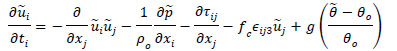
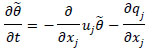
The Large Eddy Simulation (LES) has been performed using the Simulator for Wind Farm Applications (SOWFA) solver developed by the National Renewable Energy Laboratory (NREL). The LES uses ideal assumptions with a homogenous pressure gradient, flat terrain, and steady conditions (Churchfield et al. [13Churchfield M J, Moriarty P J, Vijayakumar G, Brasseur J G. Wind Energy-Related Atmospheric Boundary-Layer Large-Eddy Simulation Using OpenFOAM. Natl. Renew Energy Lab Gold CO Rep. No NRELCP-500-48905 2010., 31Churchfield MJ, Lee S, Moriarty PJ, et al. A large-eddy simulation of wind-plant aerodynamics. AIAA Pap 2012; 537: 2012.]). For the sake of completeness, the details of the solver are repeated here. The governing equations are the filtered Navier-Stokes (momentum and potential temperature transport equations) with Boussinesq approximations as follows:
 |
(1) |
 |
(2) |
 |
(3) |
where, a tilde denotes the spatially resolved filtered component at scale, denotes the modified pressure. The spatial gradient of the mean pressure term acts to drive the flow convection, (u1, u2, u3) = (u, v, w) are the components of the velocity field (u is the axial component; v is the lateral or y-component, and w is the vertical component). θ is the resolved potential temperature; θO is the reference temperature. The Subgrid Stresses (SGS) are included in the τ term along with the fluid stress tensor. The SGS flux and SFS temperature flux are parameterized, respectively as follows:
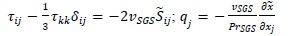 |
where D is the deviatoric SGS stress tensor; vSGS is the SGS eddy viscosity; and PrSGS is the SGS Prandtl number. The SGS flux is computed using the Moeng’s model [14Ayotte KW, Sullivan PP, Andrén A, et al. An evaluation of neutral and convective planetary boundary-layer parameterizations relative to large eddy simulations. Boundary-Layer Meteorol 1996; 79: 131-75.
[http://dx.doi.org/10.1007/BF00120078] ], where the turbulent viscosity and turbulent kinetic energy are modeled as follows:
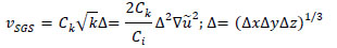 |
using the mesh cells in x, y and z directions (the resolved strain-rate tensor is) and PrSGS is constant (ref dependent on stratification level).
The finite volume solver uses the Pressure Implicit with Splitting of Operations (PISO) algorithm to solve the momentum equation [32Issa R. Solution of the implicit discretized fluid flow equations by operator splitting (PDF Download Available) Available online:
https:// www.researchgate.net/ publication/ 247576431_ Solution_of _the_ Implicit_ Discretized_ Fluid _Flow _Equations _by _Operator_ Splitting (Accessed on Dec 29, 2016).]. The pressure and velocity are solved implicitly in this method using Crank-Nicholson time advancement for the predictor and two corrector steps [13Churchfield M J, Moriarty P J, Vijayakumar G, Brasseur J G. Wind Energy-Related Atmospheric Boundary-Layer Large-Eddy Simulation Using OpenFOAM. Natl. Renew Energy Lab Gold CO Rep. No NRELCP-500-48905 2010.]. The code solves the buoyant term, the SGS viscosity, and the Coriolis terms explicitly. The pressure gradient,  , drives the flow and is constant in space. The pressure gradient is adjusted to maintain the geostrophic wind at the top of the domain. The Coriolis parameter, fc, is calculated based on the latitude, which is 40° where the NREL site is located [17Kumar V, Svensson G, Holtslag AM, Meneveau C, Parlange MB. Impact of surface flux formulations and geostrophic forcing on large-eddy simulations of diurnal atmospheric boundary layer flow. J Appl Meteorol Climatol 2010; 49: 1496-516.
[http://dx.doi.org/10.1175/2010JAMC2145.1] ]. The deviatoric SGS stress tensor,  , is equal to
  where vSGS is the SGS viscosity and
  is the resolved strain rate tensor. The SGS viscosity is modeled using the one-equation SGS model given by Moeng [4Moeng C-H. A large-eddy-simulation model for the study of planetary boundary-layer turbulence. J Atmos Sci 1984; 41: 2052-62.
[http://dx.doi.org/10.1175/1520-0469(1984)041<2052:ALESMF>2.0.CO;2] ].
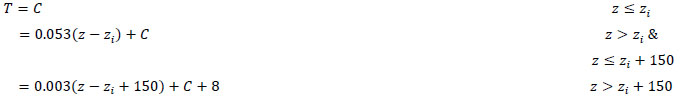
Each simulation is initialized with an initial temperature and velocity profile shown in Eq. 4. where C is a constant and is 280 for the January simulations and 300 for the July simulations. The initial temperature profile is a three-layer structure [33Sullivan PP, Patton EG. The effect of mesh resolution on convective boundary layer statistics and structures generated by large-eddy simulation. J Atmos Sci 2011; 68: 2395-415.
[http://dx.doi.org/10.1175/JAS-D-10-05010.1] ]. The first is a constant temperature gradient to the inversion height. At the initial inversion height, the temperature is changed by 8° K over 150 m. Finally, a constant temperature gradient of 0.003 Km-1 is given from the top of the inversion height to the top of the domain [13Churchfield M J, Moriarty P J, Vijayakumar G, Brasseur J G. Wind Energy-Related Atmospheric Boundary-Layer Large-Eddy Simulation Using OpenFOAM. Natl. Renew Energy Lab Gold CO Rep. No NRELCP-500-48905 2010.]. The initial velocity is prescribed as a constant geostrophic wind velocity throughout the domain. Random temperature perturbations and a sinusoidal velocity perturbation are added near the surface to decrease the amount of time to generate realistic turbulence. As the simulation progresses, the profiles develop to those of an ABL.
 |
(4) |
All lateral boundary conditions are specified as periodic. The upper-velocity boundary condition is specified as zero velocity normal to the boundary and zero gradient parallel to the boundary. A Neumann boundary is prescribed as the upper-pressure boundary condition that is determined from the normal momentum equation. The upper-temperature boundary condition is specified as a constant temperature gradient of 0.003 to match the initialized temperature profile. The upper SGS stress boundary condition is given as a zero gradient.
The surface roughness zO [8Paulson CA. The mathematical representation of wind speed and temperature profiles in the unstable atmospheric surface layer. J Appl Meteorol 1970; 9: 857-61.
[http://dx.doi.org/10.1175/1520-0450(1970)009<0857:TMROWS>2.0.CO;2] ], which represents different land and surface types, sets the lower velocity boundary condition. zO is given as 0.15 m The lower pressure boundary condition is given as the gradient determined by the normal momentum equation. The lower temperature boundary condition is given as a constant temperature flux (surface heat flux). The lower SGS viscosity boundary condition is determined using the Schumann Model [34Schumann U. Subgrid scale model for finite difference simulations of turbulent flows in plane channels and annuli. J Comput Phys 1975; 18: 376-404.
[http://dx.doi.org/10.1016/0021-9991(75)90093-5] ]. The SGS viscosity values are determined to satisfy the Schumann Model surface stress as described by Churchfield et al. [13Churchfield M J, Moriarty P J, Vijayakumar G, Brasseur J G. Wind Energy-Related Atmospheric Boundary-Layer Large-Eddy Simulation Using OpenFOAM. Natl. Renew Energy Lab Gold CO Rep. No NRELCP-500-48905 2010.].
The domain of the simulation is 4000 m x 4000 m x 2000 m. The predominant wind is set at an angle through the domain such that the large-scale structures can properly form [13Churchfield M J, Moriarty P J, Vijayakumar G, Brasseur J G. Wind Energy-Related Atmospheric Boundary-Layer Large-Eddy Simulation Using OpenFOAM. Natl. Renew Energy Lab Gold CO Rep. No NRELCP-500-48905 2010.] and the turbulent statistics did not change with increased domain size. Simulations were performed with grid points of Nx, Ny, and Nz as 160, 160 and 128 in the horizontal (x), spanwise (y), and vertical (z) - directions respectively. The grid points in the horizontal direction are equally spaced while the spacing in the vertical direction increases such that the last cell is four times larger than the first cell where Δz = .146 Nz + 5.98. The simulations were run for 9,000s and then the statistics were taken for another 2,000s (the eddy turnover times ranged from 6-12 min). Table 1 gives a list of LES cases performed for the validation. These were determined using the PDFs for surface heat flux as described in Section 3.5.

3. RESULTS AND DISCUSSION
3.1. Best Fit PDF for Surface Heat Flux
The Probability Density Functions (PDFs) are generated by grouping together surface heat flux values over a given hour, applying multiple types of PDFs to the set of data, and selecting the PDF with the best fit as determined by an R2 value [35Morgan EC, Lackner M, Vogel RM, Baise LG. Probability distributions for offshore wind speeds. Energy Convers Manage 2011; 52: 15-26.
[http://dx.doi.org/10.1016/j.enconman.2010.06.015] ]. Normal and logistic distributions were tested. The equations for the PDFs are:
 |
(5) |
 |
(6) |
where µ is the mean, σ is the standard deviation, and s is the shape parameter.
One method to validate the fits of the PDFs is by using the cumulative density function. The cumulative density function represents the probability a random variable X will be less than or equal to x. The field data is compared to the PDF, and an R2 can be determined. Fig. (6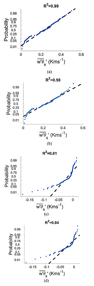 ) shows the cumulative density function fits for the PDFs of surface heat flux. Fig. (6) shows the cumulative density function fit for the (a) Normal PDF and (b) Logistic PDF using data from July at hour 12 LT. Fig. (6) also shows the cumulative density function fit for the (c) Normal PDF and (d) Logistic PDF data from July at hour 21 LT. The figure shows the 12 LT and 21 LT as representative examples for both a convective and a stable instance in the ABL. Most of the deviation between the fit and the observation occurs near the extremes of the cumulative density function. Appendix B gives a complete list of R2 values for each hour of each month. Tables 4-7 record the probability functions and their parameters at each hour for the January, May, July, and October data sets. The table shows that the normal distribution had a better fit during the convective portion of the day between 8 and 16 LT. The convective part of the day also had higher R2 values ranging from 0.93 to 0.99. The logistic distribution had a better fit during night time conditions between 18 and 6 LT. During this time the R2 values were much smaller ranging from 0.61 to 0.89 (which represents a poor fit). The convective ABL data showed a strong fit with the normal distribution. Therefore, the normal PDF was used to select discrete inputs for LES.

3.2. Selection of LES Inputs from the NREL Data
The study simulated LES cases for July 12 LT and January 12 LT using the discrete surface flux value obtained from the normal PDF. The simulations consisted of the mean, -1 standard deviation and +1 standard deviation surface heat flux for each July 12 LT and January 12 LT normal PDF. For July 12 LT the mean surface heat flux mean was 0.23 kms-1 with a standard deviation of 0.125 kms-1. The mean surface flux in January 12 LT is 0.088 kms-1 with a standard deviation was 0.06 kms-1. The July 12LT was selected because it had the largest mean surface heat flux and near the largest standard deviation. The January 12 LT was selected for comparison because the mean and standard deviation were much smaller. The correlation between boundary layer height and surface heat flux shown in Fig. (5) was then used to calculate the boundary layer height for each of the six surface heat fluxes. The boundary layer heights set the initial inversion height. Finally, the geostrophic wind was estimated using u* in the geostrophic departure described by Clarke and Hess [26Clarke RH, Hess GD. Geostrophic departure and the functions A and B of Rossby-number similarity theory. Boundary-Layer Meteorol 1974; 7: 267-87.
[http://dx.doi.org/10.1007/BF00240832] ] where the A and B coefficients are experimental values used to correct the departure function. The assumption was made to use the same values found experimentally at noon by Clarke and Hess.
The LES boundary and initial conditions for the six cases are in Table 1. The table shows the case number, the selected month and surface heat flux from the PDF, the surface heat flux used as a boundary condition, the inversion height used as an initial condition, and the geostrophic wind used to drive the flow. The table also shows the corresponding Monin-Obukhov Length from each simulation. Neutral conditions generally occur near -300 m [36Iungo GV, Porté-Agel F. Volumetric lidar scanning of wind turbine wakes under convective and neutral atmospheric stability regimes. J Atmos Ocean Technol 2014; 31: 2035-48.
[http://dx.doi.org/10.1175/JTECH-D-13-00252.1] ]. All values for the Monin-Obukhov Length fall between -20 m and -43 m and are therefore portions of the convective ABL [5Johansson C, Smedman A-S, Högström U, Brasseur JG, Khanna S. Critical test of the validity of Monin–Obukhov similarity during convective conditions. J Atmos Sci 2001; 58: 1549-66.
[http://dx.doi.org/10.1175/1520-0469(2001)058<1549:CTOTVO>2.0.CO;2] ]. The six cases cover a broad range of the data gathered from the datasets to validate the LES. The data used for validation comes by averaging the profiles of the field data that fall into bins corresponding to each simulation. The bins collect the meteorological tower data that is between 12LT-13LT of the corresponding month, ± 0.5σ of the corresponding surface heat flux, and ± 0.5 m / s of the hub height wind speed for the corresponding LES.
3.3. Validation of LES
The mean velocity and temperature profiles (not shown) matched those expected for a well-mixed convective boundary layer. The potential temperature increases near the surface for the first 100-200 m. After, the potential temperature is constant up to the inversion height where there is a sharp increase in potential temperature. The increase represents the capping inversion. Finally, the potential temperature increases at a constant rate to the top boundary. The velocity profiles have a gradient for the first 100 m. Then there is a nearly constant velocity profile to the capping inversion. At the capping inversion, there is a sharp increase in velocity to the geostrophic wind condition. These match the expected mean profile of the convective boundary layer as given by Moeng [4Moeng C-H. A large-eddy-simulation model for the study of planetary boundary-layer turbulence. J Atmos Sci 1984; 41: 2052-62.
[http://dx.doi.org/10.1175/1520-0469(1984)041<2052:ALESMF>2.0.CO;2] ].
Fig. (7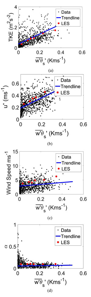 ) compares the TKE, shear exponent, wind speed, and u* obtained from LES to the NREL July 12LT data. The focus of the comparison is on the trends because the LES simulations are highly idealized. Fig. (7a) shows the correlation between surface heat flux and TKE at 74 m for the six LES simulations and the data (with a trendline). The LES simulations captured the TKE with an underprediction by less than 5% compared to the trendline. Fig. (7b) shows the correlation between surface heat flux and the friction velocity. LES overpredicted the friction velocities when compared to the trendline. The overprediction ranges from 8% to 16%, but the bias is relatively constant. The might be better estimated through a better determination of the friction length near the surface.

Fig. (7c) shows the correlation between surface heat flux and wind speed at 74 m. Although they fell within the data, the estimated geostrophic wind tended to overpredict the wind speed at 74 m. The overprediction comes from the assumption of using the same values by found experimentally by Clarke and Hess [26Clarke RH, Hess GD. Geostrophic departure and the functions A and B of Rossby-number similarity theory. Boundary-Layer Meteorol 1974; 7: 267-87.
[http://dx.doi.org/10.1007/BF00240832] ] for the A and B functions values described above (more correctly would be to calculate these values for the given datasets which are outside the scope of this work). Fig. (7d) shows the correlation between surface heat flux and wind shear. The wind shear is calculated from the wind speeds between 10 m and 86 m. The over predicted wind speed creates a similar overprediction of wind shear. Again, it is noted that the wind shear falls in the range of values measured, but tends toward the higher limit of those measured values. Fig. (7) validates the methodology of using surface heat flux from experimental data for wind turbine simulations, especially for capturing the TKE near hub height.
Further validation was performed by comparing the velocity and TKE profiles for each of the simulations generated. The NREL NWTC data is collected into bins and averaged to create the mean velocity and TKE profiles. The bins collect the meteorological tower data that is between 12LT-13LT of the corresponding month, ± 0.5σ of the corresponding surface heat flux, and ± 0.5 m/s of the hub height wind speed for the corresponding LES. Fig. (8a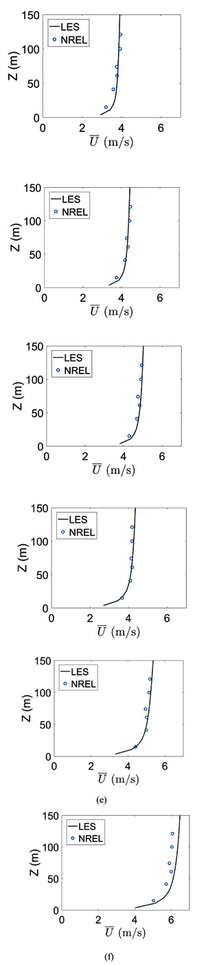 ) shows the velocity profiles for the January 12LT-1 standard deviation bin averaged data compared to the LES output. The LES output overpredicts the velocity below 50 m. Figs. (8b and 8c) shows the velocity profiles for the January mean and +1 standard deviation (respectively) bin averaged data compared to the LES output. The LES output for these two cases better predict the velocities below 50 m. The simulations capture the near uniform profiles above 50 m height that are typical for convective profiles.
Figs. (8d and 8e) show the velocity profiles for the July 12LT-1 standard deviation and mean (respectively) bin averaged data compared to the LES output. The LES output for these two cases predict the velocities below 50 m but overpredict the velocities above 50 m. Fig. (8f) shows the velocity profiles for the July 12LT +1 standard deviation bin averaged data compared to the LES output. The LES output for this case underpredicts all velocities measured from the field. Table 2 shows the error for the LES profiles compared to the binned average field data. In all simulations, the LES captures the velocity profiles well as the error falls below 5%. The small error validates the methodology for statistically selecting the boundary conditions for LES to represent day-to-day variations.
 |
Fig. (8) Velocity profile comparisons for LES and NREL bin averaged datasets for (a) Jan -1SD, (b) Jan Mean, (c) Jan +1SD, (d) Jul -1SD, (e) Jul Mean, and (f) Jul +1SD. |

Similarly, the TKE profiles for the bin-averaged NREL Dataset and the LES simulations are compared in Fig. (9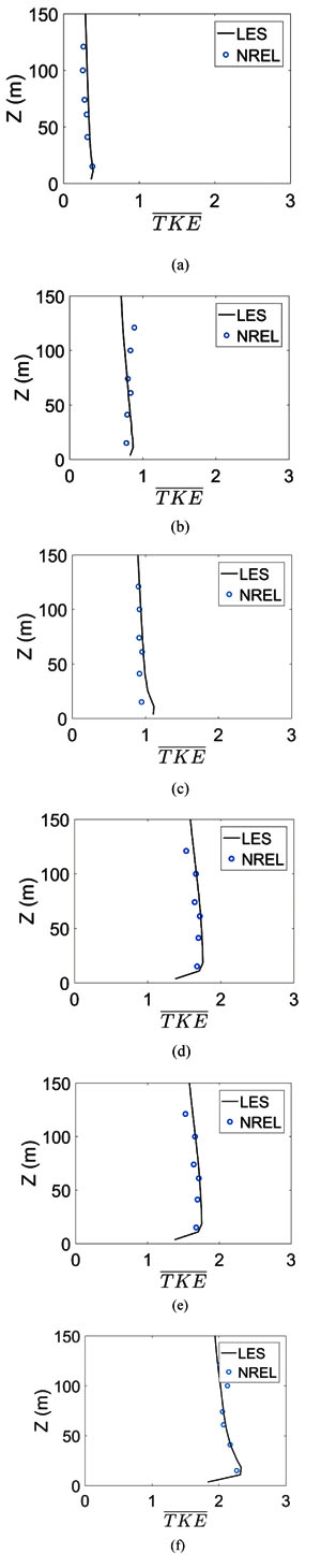 ). Fig. (9a) shows the TKE profiles for the January 12LT-1 standard deviation bin averaged data compared to the LES output. The LES underpredicts the values above 100 m. Fig. (9b) shows the TKE profiles for the January 12LT mean bin averaged data compared to the LES output. The LES underpredicts the values above 100 m and overpredicts TKE below 50 m. Fig. (9c) shows the TKE profiles for the January 12LT +1 standard deviation bin averaged data compared to the LES output. The LES overpredicts the values below 50 m but shows good agreement with all other points.
 |
Fig. (9) Velocity profile comparisons for LES and NREL bin averaged datasets for (a) Jan -1SD, (b) Jan Mean, (c) Jan +1SD, (d) Jul -1SD, (e) Jul Mean, and (f) Jul +1SD. |
Fig. (9d) shows the TKE profiles for the July 12LT -1 standard deviation bin averaged data compared to the LES output. The LES underpredicts the values above 100 m. Figs. (9e and f) show the TKE profiles for the January mean and +1 standard deviation bin averaged data compared to the LES output. The LES captures the near surface TKE well for both cases with less error above 100 m. The January 12 LT -1 standard deviation, January 12 LT Mean, and July 12 LT -1 standard deviation show small errors except for the two measurements above 100 m where the NREL data increases while the LES simulation continues to decay. The January 12LT +1 standard deviation shows a significant error at the 15 m height. The errors for the profiles are in Table 2. All errors are below 10%. The average error is 5.9% and validates that the statistically selected boundary conditions capture the TKE in the field measurements. The small error of the profiles shows that the first and second moments are obtained by using the PDF inputs for surface heat flux which further validates the methodology of creating inputs for discrete LES simulations that represent day-to-day variations in atmospheric stability.
4. DISCUSSION
Due to the computational cost of LES, it is common for wind energy applications to simulate a quasi-steady state of the atmospheric boundary layer with a specific atmospheric stability regime [37Churchfield MJ, Lee S, Michalakes J, Moriarty PJ. A numerical study of the effects of atmospheric and wake turbulence on wind turbine dynamics. J Turbul 2012; N14.
[http://dx.doi.org/10.1080/14685248.2012.668191] ]. For example, the convective ABL simulations are often conducted by selecting a surface heat flux boundary condition that characterizes a moderately convective ABL [38Ghaisas N S, Archer C L, Xie S, Wu S, Maguire E. Evaluation of layout and atmospheric stability effects in wind farms using large-eddy simulation. Wind Energy 2017.
[http://dx.doi.org/10.1002/we.2091] -40Abkar M, Porté-Agel F. Influence of atmospheric stability on wind-turbine wakes: A large-eddy simulation study. Phys Fluids 2015; 27: 035104.
[http://dx.doi.org/10.1063/1.4913695] ]. With reducing computational cost, recent work has been conducted in simulating the ABL for the entire diurnal cycle by using the hourly values of surface heat flux obtained from field measurements [16Kumar V, Kleissl J, Meneveau C, Parlange MB. Large-eddy simulation of a diurnal cycle of the atmospheric boundary layer: Atmospheric stability and scaling issues. Water Resour Res 2006; 42: W06D09.
[http://dx.doi.org/10.1029/2005WR004651] , 18Basu S, Vinuesa J-F, Swift A. Dynamic LES modeling of a diurnal cycle. J Appl Meteorol Climatol 2008; 47: 1156-74.
[http://dx.doi.org/10.1175/2007JAMC1677.1] ]. It is becoming increasingly possible to conduct LES for the entire diurnal cycle even for wind turbine applications. LES was conducted for an idealized finite wind farm for a complete diurnal cycle [20Abkar M, Sharifi A, Porté-Agel F. Wake flow in a wind farm during a diurnal cycle. J Turbul 2016; 17: 420-41.
[http://dx.doi.org/10.1080/14685248.2015.1127379] ], and the results showed that the power deficit increased from 28% in the most convective conditions to 58% under the most stable conditions. However, it is still not computationally feasible to perform LES to obtain a monthly energy estimate required for evaluating wind potential of wind farm sites [41Celik AN. A statistical analysis of wind power density based on the Weibull and Rayleigh models at the southern region of Turkey. Renew Energy 2004; 29: 593-604.
[http://dx.doi.org/10.1016/j.renene.2003.07.002] -43García-Bustamante E, González-Rouco JF, Jiménez PA, Navarro J, Montávez JP. A comparison of methodologies for monthly wind energy estimation. Wind Energy Int J Prog Appl Wind Power Convers Technol 2009; 12: 640-59.]. In particular, variations in atmospheric stability at larger timescales (i.e., across multiple days in a month) are not always accounted for during modeling [44Barthelmie RJ, Pryor SC, Frandsen ST, et al. Quantifying the impact of wind turbine wakes on power output at offshore wind farms. J Atmos Ocean Technol 2010; 27: 1302-17.
[http://dx.doi.org/10.1175/2010JTECHA1398.1] ].
The current study proposes a novel direction for accounting the day-to-day variations in the atmospheric stability into the LES model. The variations are simulated as separate discrete LES. This methodology is similar to Monte Carlo probability theory. Monte Carlo probability uses PDFs from data to generate inputs used for discrete simulations [45James F. Monte Carlo theory and practice. Rep Prog Phys 1980; 43: 1145.
[http://dx.doi.org/10.1088/0034-4885/43/9/002] , 46Metropolis N, Ulam S. The Monte Carlo method. J Am Stat Assoc 1949; 44(247): 335-41.
[http://dx.doi.org/10.1080/01621459.1949.10483310] [PMID: 18139350] ]. The outputs of the discrete simulations help quantify the range of possible outcomes based on the variability of inputs [47Hrafnkelsson B, Oddsson GV, Unnthorsson R. A Method for estimating annual energy production using Monte Carlo Wind speed simulation. Energies 2016; 9: 286.
[http://dx.doi.org/10.3390/en9040286] ]. Although the current study does not generate the number of LES required for a complete Monte Carlo simulation [48Binder K. Introduction: Theory and “technical” aspects of Monte Carlo simulations.Monte Carlo Methods in Statistical Physics 1986; 1-45.
[http://dx.doi.org/10.1007/978-3-642-82803-4_1] ], the idea is still the same. The PDF is used to generate discrete inputs for LES (selected as the mean +1 standard deviation, and -1 standard deviation). The discrete outputs from the LES help quantify the variability in the outputs base on the variability of the inputs. The study uses high-resolution data from the NREL NWTC database to build a monthly averaged PDF of surface heat flux at each hour of the day for each month. The PDF is used to select the LES inputs at each hour, particularly the mean, +1 standard deviation, and -1 standard deviation and their corresponding initial inversion heights and geostrophic winds. The inversion height was selected based on the correlation between surface heat flux and ABL height as shown in Fig. (5). The geostrophic wind was selected using the geostrophic departure function from Clarke and Hess [26Clarke RH, Hess GD. Geostrophic departure and the functions A and B of Rossby-number similarity theory. Boundary-Layer Meteorol 1974; 7: 267-87.
[http://dx.doi.org/10.1007/BF00240832] ]. The PDF is also used to collect the field data into bins for validation. The study focuses on the PDF for July 12 LT because it had the largest mean surface heat flux and standard deviation from the mean. The study also included the January 12 LT PDF for comparisons because it had a much smaller mean surface heat flux and standard deviation.
The best fit PDF for the convective portion of the ABL was the normal distribution, which matches models of the surface heat flux for near-neutral conditions [49Katul GG. A model for sensible heat flux probability density function for near-neutral and slightly-stable atmospheric flows. Boundary-Layer Meteorol 1994; 71: 1-20.
[http://dx.doi.org/10.1007/BF00709217] ]. The mean of the PDF is the expected value of the function over the entire month at each hour. The standard deviation represents the variation that occurs at each hour of the month. The difference between the +1 standard deviation and -1 standard deviation represents 68% of the data. The field data was collected into bins that correspond to each simulation. The bins collect the meteorological tower data that is between 12 -13LT of the corresponding month, ± 0.5 σ of the corresponding surface heat flux, and ± 0.5 m / s of the hub height wind speed for the corresponding LES. The binned metrological data were averaged to generate vertical profiles of velocity and TKE.
LES was conducted to simulate the case of January 12LT and July 12LT by using the mean value of PDFs of surface flux as discrete boundary conditions. For all the simulations, the initial inversion height was selected using the correlation between surface heat flux and boundary height measured in the field data. The geostrophic wind was estimated using u* with the geostrophic departure described by Clarke and Hess [26Clarke RH, Hess GD. Geostrophic departure and the functions A and B of Rossby-number similarity theory. Boundary-Layer Meteorol 1974; 7: 267-87.
[http://dx.doi.org/10.1007/BF00240832] ]. The mean July simulation had a higher hub height wind speed (5.0vs. 4.2 m/s), and TKE (1.4vs. 0.7 m2/s2) than the January mean simulation. Two additional LES were conducted by using -1 standard deviation, and + 1 standard deviation from mean values of PDF of surface flux as inputs into LES. The July +1 standard deviation simulation had a hub height TKE of 1.7 m2/s2 while the -1 standard deviation simulation was 0.9 m2/s2. The increased surface heat flux increased the hub height TKE by 2 times. The difference in the January +1 standard deviation and -1 standard deviation was 0.35 m2/s2 and 0.95 m2/s2. The day-to-day variations in surface heat flux had significant impacts on the outputs of LES. These wide variations in TKE flux have considerable impacts on wind turbine performance [22Wu Y-T, Porté-Agel F. Atmospheric turbulence effects on wind-turbine wakes: An LES study. Energies 2012; 5: 5340-62.
[http://dx.doi.org/10.3390/en5125340] , 24Clifton A, Schreck S, Scott G, Kelley N, Lundquist JK. Turbine inflow characterization at the national wind technology center. J Sol Energy Eng 2013; 135: 031017-031017-11.
[http://dx.doi.org/10.1115/1.4024068] , 36Iungo GV, Porté-Agel F. Volumetric lidar scanning of wind turbine wakes under convective and neutral atmospheric stability regimes. J Atmos Ocean Technol 2014; 31: 2035-48.
[http://dx.doi.org/10.1175/JTECH-D-13-00252.1] ].
The outputs of the six LES captured the same correlation of surface heat flux with TKE, wind speed, wind shear, and friction velocity at hub height as the field measurements. The LES correlation between surface heat flux and TKE showed that for every increase in 0.1 kms-1 the TKE increased by 0.42 m2/s2. The LES correlations showed an increase in friction velocity and wind speed of 0.095 m/s and 0.74 m/s for every increase in 0.1 kms-1. The correlations show the significant impact to LES outputs due to the variation in surface heat flux. Using the methodology described the discrete LES were able to capture these variations using discrete LES.
The binned average velocity and TKE profiles validated the LES. The LES profiles matched the velocity profiles with 4% error and the TKE profiles to 6% error on average. The results are promising and demonstrate the methodology approach is robust enough to capture the ABL turbulence over multiple diurnal cycles. The current work is an important direction for futuristic LES studies of wind turbines in ABL based on field measurements. The significance of the results is two folds (a) Day-to-day variability of surface heat flux is well-represented in TKE and ABL depth, hence surface heat flux is a boundary condition that dictates the efficacy of LES in capturing the day-to-day variation of ABL turbulence, and (b) The methodology allows the outputs from LES to represent mathematically significant variations that occur in the atmosphere. Applications of LES, such as wind turbine simulations, can use the methodology to quantify the variability in turbine performance based on the day-to-day variations of surface heat flux. These predictions add further fidelity to wind turbine LES. The study serves as a validation incorporate field measurements averaged over multiple diurnal cycles into LES applications.
CONCLUSION AND RECOMMENDATION
The current study proposes a methodology to conduct discrete LES that represents day-to-day variations in atmospheric stability using realistic boundary conditions from field data. The NREL NWTC field measurements have demonstrated surface heat flux exhibits significant day-day variations. For July 12 LT, the surface heat flux had a mean of 0.23 kms-1 and a standard deviation of 0.124 kms-1. The wide range of surface heat flux impacts the output of LES with significant changes in TKE. The best fit PDF for the convective surface heat flux data was the normal PDF (R2 values above 0.93 for all hours). The methodology used the January 12LT and July 12LT to select the mean, +1 standard deviation, and -1 standard deviation surface heat fluxes for LES (six total simulations). These represent the day-to-day variations that occur at 12LT. Each surface heat flux has a corresponding initial inversion height and geostrophic wind used as additional inputs for the LES. The LES outputs were validated to the velocity and TKE profiles. The average errors of the six simulations were 4% for velocity and 6% for TKE. The validation shows the robustness of the methodology to capture realistic velocity and TKE over day-to-day variations of surface heat flux. The six simulations also match similar trends in TKE, friction velocity, wind speed, and wind shear measured from the field.
There are many applications where the current methodology could be applied. These include LES of wind turbine performance, wind turbine wake decay, plume dispersion, and spreading of forest fires, all of which are highly dependent on variations in stability. For each of the examples above, the mean, +1 standard deviation, and -1 standard deviation cases would represent a range of probable occurrences over the monthly averaged conditions. This will help to better understand variations of the outputs of LES (i.e., wake decay or plume dispersion) based on expected variations in the field.
The current study assumed an inversion height and geostrophic wind for each surface heat flux, which allowed the inputs to be selected from a single surface heat flux PDF. The next natural step to improve the methodology would be to incorporate multivariate PDFs to generate the inputs into LES. For example, a bivariate PDF might include wind speed (through the geostrophic wind) and surface heat flux. A multivariate PDF would increase the number of simulations required, but would also include more than just the variability from surface heat flux. However, a multivariate PDF is expected to make the methodology even more robust.
ETHICS APPROVAL AND CONSENT TO PARTICIPATE
Not applicable.
HUMAN AND ANIMAL RIGHTS
No animals/ humans were used for the studies that are basis of this research.
CONSENT FOR PUBLICATION
Not applicable.
CONFLICT OF INTEREST
The authors declare no conflict of interest, financial or otherwise.
ACKNOWLEDGEMENTS
The authors would like to acknowledge the Texas Advanced Computing Center for the computer time to perform the simulations. The Authors would like to acknowledge the National Renewable Energy Lab for collecting and giving the data from the field site as well as developing the SOWFA code.
APPENDIX A
ABL Metrics
Appendix A give the ABL metrics parameters descriped in the methodology section: The ABL parameters measured and their respective heights for both data sets. The devices used for capturing the NREL data sets are shown in [24Clifton A, Schreck S, Scott G, Kelley N, Lundquist JK. Turbine inflow characterization at the national wind technology center. J Sol Energy Eng 2013; 135: 031017-031017-11.
[http://dx.doi.org/10.1115/1.4024068] , 27 NWTC Information Portal (NWTC 135-m Meteorological Towers Data Repository).
https:// nwtc.nrel.gov/ 135mData Last modified 01-April-2015 ; Accessed 21-October-2018.].
The three components of the velocity (u, v and w) and temperature (T) are averaged over ten minutes. The averaged quantities are then used to determine the velocity fluctuations (u’, v’, w’) and temperature fluctuation (T') over the ten-minute period. Turbulence characteristics, including, turbulence kinetic energy (TKE), friction velocity, and second order turbulence statistics are calculated as described by Clifton [29Sugiyama G, Nasstrom JS. Methods for determining the height of the atmospheric boundary layer. Lawrence Livermore Natl. Lab Intern Rep UCRL-ID-133200 1999.].
The turbulent kinetic energy (TKE) is a measure of the amount of energy based on the fluctuations from eddies. It includes production from buoyancy and shear, dissipation by viscous motions, and transport by turbulent and pressure terms [50Wyngaard JC, Coté OR. The budgets of turbulent kinetic energy and temperature variance in the atmospheric surface layer. J Atmos Sci 1971; 28: 190-201.
[http://dx.doi.org/10.1175/1520-0469(1971)028<0190:TBOTKE>2.0.CO;2] ]. The mean TKE over the ten-minute time period is calculated in Eq. (7).
The turbulent fluctuations are then used to determine the friction velocity, or velocity scale u* [3Stull RB. An introduction to boundary layer meteorology 2012; Vol. 13]. The friction velocity (u*) is a velocity scale derived from the wall shear-stress. The friction velocity is calculated using the covariance [51Weber RO. Remarks on the definition and estimation of friction velocity. Boundary-Layer Meteorol 1999; 93: 197-209.
[http://dx.doi.org/10.1023/A:1002043826623] ] in eq. (8)
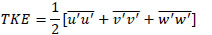 |
(7) |
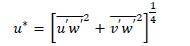 |
(8) |
The convective temperature scale is also calculated with the turbulent fluctuations. The calculation uses two assumptions. First, the temperature fluctuation is approximately the potential temperature fluctuation near the surface [27 NWTC Information Portal (NWTC 135-m Meteorological Towers Data Repository).
https:// nwtc.nrel.gov/ 135mData Last modified 01-April-2015 ; Accessed 21-October-2018.]. Second, that the sonic temperature fluctuation is approximately the virtual temperature fluctuation [52Kaimal JC, Gaynor JE. Another look at sonic thermometry. Boundary-Layer Meteorol 1991; 56: 401-10.
[http://dx.doi.org/10.1007/BF00119215] ]. With those assumptions, the temperature scale is
 |
(9) |
The potential temperature (θ) is the temperature of a parcel if it were adiabatically brought to a reference pressure [3Stull RB. An introduction to boundary layer meteorology 2012; Vol. 13]. The reference pressure is 1000 hPa the gas constant R is given as 0.286 kJ kg-1K-1 and the specific heat Cp as 1.005 kJ kg-1K-1. In addition, the virtual temperature is also calculated in Eq. (11) to include the moisture in the air. r is the mixing ratio of water vapor in the air and r1 is the mixing ratio of liquid water in the air.
 |
(10) |
 |
(11) |
The wind profile of the atmospheric boundary layer is generally approximated as power law with an exponent α that represents the vertical gradient in the wind speed, which is referred to as the shear [24Clifton A, Schreck S, Scott G, Kelley N, Lundquist JK. Turbine inflow characterization at the national wind technology center. J Sol Energy Eng 2013; 135: 031017-031017-11.
[http://dx.doi.org/10.1115/1.4024068] , 53Wharton S, Lundquist JK. Assessing atmospheric stability and its impacts on rotor-disk wind characteristics at an onshore wind farm. Wind Energy (Chichester Engl) 2012; 15: 525-46.
[http://dx.doi.org/10.1002/we.483] , 54St Martin CM, Lundquist JK, Clifton A, Poulos GS, Schreck SJ. Wind turbine power production and annual energy production depend on atmospheric stability and turbulence. Wind Energy Sci 2016; 1: 221.
[http://dx.doi.org/10.5194/wes-1-221-2016] ]. The values of α are determined from two levels of wind velocity, U, at heights z and zO as follows:
 |
(12) |
The stability of the atmosphere is determined using three different methods: Method (1): The atmospheric stability is expressed in terms of Monin-Obukhov length (L), which is a parameter that expresses the roles of buoyancy and shear based on the gravity acceleration, friction velocity, von Karman constant k (given as 0.4), and kinematic heat flux to create a ratio of the relative roles of shear and buoyancy [30Foken T. 50 years of the Monin–Obukhov similarity theory. Boundary-Layer Meteorol 2006; 119: 431-47.
[http://dx.doi.org/10.1007/s10546-006-9048-6] ]. The ratio is
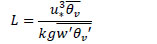 |
(13) |
The kinematic heat flux  is approximated as
  because the turbulent fluctuations measured from a sonic anemometer approximate the turbulent component of the virtual potential temperature. The Monin-Obukhov Length is negative for unstable conditions and positive for stable conditions.
In method (2): The gradient Richardson number is a measure of the atmospheric stability using temperature and velocity gradients. It is a dimensionless value that is related to the buoyancy production and shear production [55Businger JA, Wyngaard JC, Izumi Y, Bradley EF. Flux-profile relationships in the atmospheric surface layer. J Atmos Sci 1971; 28: 181-9.
[http://dx.doi.org/10.1175/1520-0469(1971)028<0181:FPRITA>2.0.CO;2] ] and is calculated as
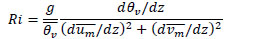 |
(14) |
In method (3): The Speed Richardson Number is also used [24Clifton A, Schreck S, Scott G, Kelley N, Lundquist JK. Turbine inflow characterization at the national wind technology center. J Sol Energy Eng 2013; 135: 031017-031017-11.
[http://dx.doi.org/10.1115/1.4024068] , 27 NWTC Information Portal (NWTC 135-m Meteorological Towers Data Repository).
https:// nwtc.nrel.gov/ 135mData Last modified 01-April-2015 ; Accessed 21-October-2018.]. The Speed Richardson Number uses the total horizontal wind speed gradient rather than using the and components [56Byun DW. On the analytical solutions of flux-profile relationships for the atmospheric surface layer. J Appl Meteorol 1990; 29: 652-7.
[http://dx.doi.org/10.1175/1520-0450(1990)029<0652:OTASOF>2.0.CO;2] ] and is
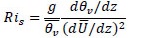 |
(15) |
Sugiyama and Nasstrom [29Sugiyama G, Nasstrom JS. Methods for determining the height of the atmospheric boundary layer. Lawrence Livermore Natl. Lab Intern Rep UCRL-ID-133200 1999.] explained the different methods for estimating the boundary layer height (habl) based on friction velocities. These include those developed by Blackadar and Tennekes [57Blackadar AK, Tennekes H. Asymptotic similarity in neutral barotropic planetary boundary layers. J Atmos Sci 1968; 25: 1015-20.
[http://dx.doi.org/10.1175/1520-0469(1968)025<1015:ASINBP>2.0.CO;2] ] for stable conditions and slab models such as those developed by Tennekes [58Tennekes H. A model for the dynamics of the inversion above a convective boundary layer. J Atmos Sci 1973; 30: 558-67.
[http://dx.doi.org/10.1175/1520-0469(1973)030<0558:AMFTDO>2.0.CO;2] ] and Carson [6Carson DJ. The development of a dry inversion-capped convectively unstable boundary layer. Q J R Meteorol Soc 1973; 99: 450-67.
[http://dx.doi.org/10.1002/qj.49709942105] ]. This analysis assumes the fluxes depend only upon u* and the Coriolis parameter fc for simplicity as
 |
(16) |
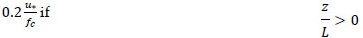 |
(17) |
Clake and Hess [26Clarke RH, Hess GD. Geostrophic departure and the functions A and B of Rossby-number similarity theory. Boundary-Layer Meteorol 1974; 7: 267-87.
[http://dx.doi.org/10.1007/BF00240832] ] described a method to estimate the geostrophic wind based on departure functions A and B that are determined empirically. There experimental values for A and B were used with equations 18 and 19 to estimate the geostrophic wind where ug and vg are the horizontal components of geostrophic wind.
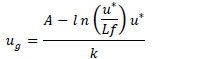 |
(18) |
 |
(19) |
APPENDIX B
Appendix B gives the complete results for all probability density functions found during the analysis. These are given in Tables 3-7. For each data set, the Normal Distribution is given for each hour. In addition, if there is a better fit found, that distribution is also given with its name and parameters (given as A and B).


REFERENCES
| [1] | Carruthers DJ, Holroyd RJ, Hunt JCR, et al. UK-ADMS: A new approach to modelling dispersion in the earth’s atmospheric boundary layer. J Wind Eng Ind Aerodyn 1994; 52: 139-53. [http://dx.doi.org/10.1016/0167-6105(94)90044-2] |
| [2] | Smirnova TG, Brown JM, Benjamin SG. Performance of different soil model configurations in simulating ground surface temperature and surface fluxes. Mon Weather Rev 1997; 125: 1870-84. [http://dx.doi.org/10.1175/1520-0493(1997)125<1870:PODSMC>2.0.CO;2] |
| [3] | Stull RB. An introduction to boundary layer meteorology 2012; Vol. 13 |
| [4] | Moeng C-H. A large-eddy-simulation model for the study of planetary boundary-layer turbulence. J Atmos Sci 1984; 41: 2052-62. [http://dx.doi.org/10.1175/1520-0469(1984)041<2052:ALESMF>2.0.CO;2] |
| [5] | Johansson C, Smedman A-S, Högström U, Brasseur JG, Khanna S. Critical test of the validity of Monin–Obukhov similarity during convective conditions. J Atmos Sci 2001; 58: 1549-66. [http://dx.doi.org/10.1175/1520-0469(2001)058<1549:CTOTVO>2.0.CO;2] |
| [6] | Carson DJ. The development of a dry inversion-capped convectively unstable boundary layer. Q J R Meteorol Soc 1973; 99: 450-67. [http://dx.doi.org/10.1002/qj.49709942105] |
| [7] | Bhaganagar K, Debnath M. The effects of mean atmospheric forcings of the stable atmospheric boundary layer on wind turbine wake. J Renew Sustain Energy 2015; 7: 013124. [http://dx.doi.org/10.1063/1.4907687] |
| [8] | Paulson CA. The mathematical representation of wind speed and temperature profiles in the unstable atmospheric surface layer. J Appl Meteorol 1970; 9: 857-61. [http://dx.doi.org/10.1175/1520-0450(1970)009<0857:TMROWS>2.0.CO;2] |
| [9] | Barr AG, Betts AK. Radiosonde boundary layer budgets above a boreal forest. J Geophys Res Atmos 1997; 102: 29205-12. [http://dx.doi.org/10.1029/97JD01105] |
| [10] | Barr AG, Betts AK, Desjardins RL, MacPherson JI. Comparison of regional surface fluxes from boundary-layer budgets and aircraft measurements above boreal forest. J Geophys Res Atmos 1997; 102: 29213-8. [http://dx.doi.org/10.1029/97JD01104] |
| [11] | Grimmond CSB, Oke TR. Comparison of heat fluxes from summertime observations in the suburbs of four North American cities. J Appl Meteorol 1995; 34: 873-89. [http://dx.doi.org/10.1175/1520-0450(1995)034<0873:COHFFS>2.0.CO;2] |
| [12] | Yusuf N, Okoh D, Musa I, Adedoja S, Said R. A study of the surface air temperature variations in Nigeria. Open Atmos Sci J 2017; 11: 54-70. |
| [13] | Churchfield M J, Moriarty P J, Vijayakumar G, Brasseur J G. Wind Energy-Related Atmospheric Boundary-Layer Large-Eddy Simulation Using OpenFOAM. Natl. Renew Energy Lab Gold CO Rep. No NRELCP-500-48905 2010. |
| [14] | Ayotte KW, Sullivan PP, Andrén A, et al. An evaluation of neutral and convective planetary boundary-layer parameterizations relative to large eddy simulations. Boundary-Layer Meteorol 1996; 79: 131-75. [http://dx.doi.org/10.1007/BF00120078] |
| [15] | Maldaner S, Degrazia AG, Rizza U. Derivation of the turbulent time scales and velocity variances from lES spectral data: Application in a lagrangian stochastic dispersion model. Open Atmos Sci J 2014; 8: 16-21. |
| [16] | Kumar V, Kleissl J, Meneveau C, Parlange MB. Large-eddy simulation of a diurnal cycle of the atmospheric boundary layer: Atmospheric stability and scaling issues. Water Resour Res 2006; 42: W06D09. [http://dx.doi.org/10.1029/2005WR004651] |
| [17] | Kumar V, Svensson G, Holtslag AM, Meneveau C, Parlange MB. Impact of surface flux formulations and geostrophic forcing on large-eddy simulations of diurnal atmospheric boundary layer flow. J Appl Meteorol Climatol 2010; 49: 1496-516. [http://dx.doi.org/10.1175/2010JAMC2145.1] |
| [18] | Basu S, Vinuesa J-F, Swift A. Dynamic LES modeling of a diurnal cycle. J Appl Meteorol Climatol 2008; 47: 1156-74. [http://dx.doi.org/10.1175/2007JAMC1677.1] |
| [19] | Lee JC, Lundquist JK. Observing and simulating wind-turbine wakes during the evening transition 2017; 1-26. |
| [20] | Abkar M, Sharifi A, Porté-Agel F. Wake flow in a wind farm during a diurnal cycle. J Turbul 2016; 17: 420-41. [http://dx.doi.org/10.1080/14685248.2015.1127379] |
| [21] | Abkar M, Porté-Agel F. Influence of atmospheric stability on wind-turbine wakes: A large-eddy simulation study. Phys Fluids 2015; 27: 035104. [http://dx.doi.org/10.1063/1.4913695] |
| [22] | Wu Y-T, Porté-Agel F. Atmospheric turbulence effects on wind-turbine wakes: An LES study. Energies 2012; 5: 5340-62. [http://dx.doi.org/10.3390/en5125340] |
| [23] | Chamorro LP, Porté-Agel F. A wind-tunnel investigation of wind-turbine wakes: Boundary-layer turbulence effects. Boundary-Layer Meteorol 2009; 132: 129-49. [http://dx.doi.org/10.1007/s10546-009-9380-8] |
| [24] | Clifton A, Schreck S, Scott G, Kelley N, Lundquist JK. Turbine inflow characterization at the national wind technology center. J Sol Energy Eng 2013; 135: 031017-031017-11. [http://dx.doi.org/10.1115/1.4024068] |
| [25] | Clifton A. An unofficial guide to data products from the NWTC 135-m Meteorological Towers 2007. |
| [26] | Clarke RH, Hess GD. Geostrophic departure and the functions A and B of Rossby-number similarity theory. Boundary-Layer Meteorol 1974; 7: 267-87. [http://dx.doi.org/10.1007/BF00240832] |
| [27] | NWTC Information Portal (NWTC 135-m Meteorological Towers Data Repository). https:// nwtc.nrel.gov/ 135mData Last modified 01-April-2015 ; Accessed 21-October-2018. |
| [28] | Hogg RV, Craig AT. Introduction to mathematical statistics(5th edition) 1995. |
| [29] | Sugiyama G, Nasstrom JS. Methods for determining the height of the atmospheric boundary layer. Lawrence Livermore Natl. Lab Intern Rep UCRL-ID-133200 1999. |
| [30] | Foken T. 50 years of the Monin–Obukhov similarity theory. Boundary-Layer Meteorol 2006; 119: 431-47. [http://dx.doi.org/10.1007/s10546-006-9048-6] |
| [31] | Churchfield MJ, Lee S, Moriarty PJ, et al. A large-eddy simulation of wind-plant aerodynamics. AIAA Pap 2012; 537: 2012. |
| [32] | Issa R. Solution of the implicit discretized fluid flow equations by operator splitting (PDF Download Available) Available online: https:// www.researchgate.net/ publication/ 247576431_ Solution_of _the_ Implicit_ Discretized_ Fluid _Flow _Equations _by _Operator_ Splitting (Accessed on Dec 29, 2016). |
| [33] | Sullivan PP, Patton EG. The effect of mesh resolution on convective boundary layer statistics and structures generated by large-eddy simulation. J Atmos Sci 2011; 68: 2395-415. [http://dx.doi.org/10.1175/JAS-D-10-05010.1] |
| [34] | Schumann U. Subgrid scale model for finite difference simulations of turbulent flows in plane channels and annuli. J Comput Phys 1975; 18: 376-404. [http://dx.doi.org/10.1016/0021-9991(75)90093-5] |
| [35] | Morgan EC, Lackner M, Vogel RM, Baise LG. Probability distributions for offshore wind speeds. Energy Convers Manage 2011; 52: 15-26. [http://dx.doi.org/10.1016/j.enconman.2010.06.015] |
| [36] | Iungo GV, Porté-Agel F. Volumetric lidar scanning of wind turbine wakes under convective and neutral atmospheric stability regimes. J Atmos Ocean Technol 2014; 31: 2035-48. [http://dx.doi.org/10.1175/JTECH-D-13-00252.1] |
| [37] | Churchfield MJ, Lee S, Michalakes J, Moriarty PJ. A numerical study of the effects of atmospheric and wake turbulence on wind turbine dynamics. J Turbul 2012; N14. [http://dx.doi.org/10.1080/14685248.2012.668191] |
| [38] | Ghaisas N S, Archer C L, Xie S, Wu S, Maguire E. Evaluation of layout and atmospheric stability effects in wind farms using large-eddy simulation. Wind Energy 2017. [http://dx.doi.org/10.1002/we.2091] |
| [39] | Xie S, Archer CL. A numerical study of wind-turbine wakes for three atmospheric stability conditions 2017; 1-26. |
| [40] | Abkar M, Porté-Agel F. Influence of atmospheric stability on wind-turbine wakes: A large-eddy simulation study. Phys Fluids 2015; 27: 035104. [http://dx.doi.org/10.1063/1.4913695] |
| [41] | Celik AN. A statistical analysis of wind power density based on the Weibull and Rayleigh models at the southern region of Turkey. Renew Energy 2004; 29: 593-604. [http://dx.doi.org/10.1016/j.renene.2003.07.002] |
| [42] | Keyhani A, Ghasemi-Varnamkhasti M, Khanali M, Abbaszadeh R. An assessment of wind energy potential as a power generation source in the capital of Iran, Tehran. Energy 2010; 35: 188-201. [http://dx.doi.org/10.1016/j.energy.2009.09.009] |
| [43] | García-Bustamante E, González-Rouco JF, Jiménez PA, Navarro J, Montávez JP. A comparison of methodologies for monthly wind energy estimation. Wind Energy Int J Prog Appl Wind Power Convers Technol 2009; 12: 640-59. |
| [44] | Barthelmie RJ, Pryor SC, Frandsen ST, et al. Quantifying the impact of wind turbine wakes on power output at offshore wind farms. J Atmos Ocean Technol 2010; 27: 1302-17. [http://dx.doi.org/10.1175/2010JTECHA1398.1] |
| [45] | James F. Monte Carlo theory and practice. Rep Prog Phys 1980; 43: 1145. [http://dx.doi.org/10.1088/0034-4885/43/9/002] |
| [46] | Metropolis N, Ulam S. The Monte Carlo method. J Am Stat Assoc 1949; 44(247): 335-41. [http://dx.doi.org/10.1080/01621459.1949.10483310] [PMID: 18139350] |
| [47] | Hrafnkelsson B, Oddsson GV, Unnthorsson R. A Method for estimating annual energy production using Monte Carlo Wind speed simulation. Energies 2016; 9: 286. [http://dx.doi.org/10.3390/en9040286] |
| [48] | Binder K. Introduction: Theory and “technical” aspects of Monte Carlo simulations.Monte Carlo Methods in Statistical Physics 1986; 1-45. [http://dx.doi.org/10.1007/978-3-642-82803-4_1] |
| [49] | Katul GG. A model for sensible heat flux probability density function for near-neutral and slightly-stable atmospheric flows. Boundary-Layer Meteorol 1994; 71: 1-20. [http://dx.doi.org/10.1007/BF00709217] |
| [50] | Wyngaard JC, Coté OR. The budgets of turbulent kinetic energy and temperature variance in the atmospheric surface layer. J Atmos Sci 1971; 28: 190-201. [http://dx.doi.org/10.1175/1520-0469(1971)028<0190:TBOTKE>2.0.CO;2] |
| [51] | Weber RO. Remarks on the definition and estimation of friction velocity. Boundary-Layer Meteorol 1999; 93: 197-209. [http://dx.doi.org/10.1023/A:1002043826623] |
| [52] | Kaimal JC, Gaynor JE. Another look at sonic thermometry. Boundary-Layer Meteorol 1991; 56: 401-10. [http://dx.doi.org/10.1007/BF00119215] |
| [53] | Wharton S, Lundquist JK. Assessing atmospheric stability and its impacts on rotor-disk wind characteristics at an onshore wind farm. Wind Energy (Chichester Engl) 2012; 15: 525-46. [http://dx.doi.org/10.1002/we.483] |
| [54] | St Martin CM, Lundquist JK, Clifton A, Poulos GS, Schreck SJ. Wind turbine power production and annual energy production depend on atmospheric stability and turbulence. Wind Energy Sci 2016; 1: 221. [http://dx.doi.org/10.5194/wes-1-221-2016] |
| [55] | Businger JA, Wyngaard JC, Izumi Y, Bradley EF. Flux-profile relationships in the atmospheric surface layer. J Atmos Sci 1971; 28: 181-9. [http://dx.doi.org/10.1175/1520-0469(1971)028<0181:FPRITA>2.0.CO;2] |
| [56] | Byun DW. On the analytical solutions of flux-profile relationships for the atmospheric surface layer. J Appl Meteorol 1990; 29: 652-7. [http://dx.doi.org/10.1175/1520-0450(1990)029<0652:OTASOF>2.0.CO;2] |
| [57] | Blackadar AK, Tennekes H. Asymptotic similarity in neutral barotropic planetary boundary layers. J Atmos Sci 1968; 25: 1015-20. [http://dx.doi.org/10.1175/1520-0469(1968)025<1015:ASINBP>2.0.CO;2] |
| [58] | Tennekes H. A model for the dynamics of the inversion above a convective boundary layer. J Atmos Sci 1973; 30: 558-67. [http://dx.doi.org/10.1175/1520-0469(1973)030<0558:AMFTDO>2.0.CO;2] |