- Home
- About Journals
-
Information for Authors/ReviewersEditorial Policies
Publication Fee
Publication Cycle - Process Flowchart
Online Manuscript Submission and Tracking System
Publishing Ethics and Rectitude
Authorship
Author Benefits
Reviewer Guidelines
Guest Editor Guidelines
Peer Review Workflow
Quick Track Option
Copyediting Services
Bentham Open Membership
Bentham Open Advisory Board
Archiving Policies
Fabricating and Stating False Information
Post Publication Discussions and Corrections
Editorial Management
Advertise With Us
Funding Agencies
Rate List
Kudos
General FAQs
Special Fee Waivers and Discounts
- Contact
- Help
- About Us
- Search


The Open Petroleum Engineering Journal
(Discontinued)
ISSN: 1874-8341 ― Volume 12, 2019
Modelling of Sub-Sea Gas Transmission Pipeline to Predict Insulation Failure
Ode Samson Chinedu1, Okoro Emeka Emmanuel2, *, Ekeinde Evelyn Bose1, Dosunmu Adewale1
Abstract
Background:
Thermally insulated subsea production and transmission systems are becoming more common in deep-water/ offshore operations. Premature failures of the insulation materials for these gas transmission pipelines have had significant operational impacts. The ability to timely detect these failures within these systems has been a very difficult task for the oil and gas industries. Thus, periodic survey of the subsea transmission systems is the present practice. In addition, a new technology called optic-fibre Distributed Temperature Sensing system (DTS) is now being used to monitor subsea transmission pipeline temperatures; but this technology is rather very expensive.
Objective:
However, this study proposed a model which will not only predict premature insulation failure in these transmission pipelines; but will also predict the section of the transmission line where the failure had occurred.
Methods:
From this study, we deduced that in gas pipeline flow, exit temperature for the system increases exponentially with the distance of insulation failure and approaches the normal operation if the failure occurs towards the exit of the gas pipe. This model can also be used to check the readings of an optic-fibre distributed temperature sensors.
Result and Conclusion:
After developing this model using classical visual basic and excel package, the model was validated by cross plotting the normal temperature profiles of the model and field data; and R-factor of 0.967 was obtained. Analysis of the results obtained from the model showed that insulation failure in subsea gas transmission pipeline can be predicted on a real-time basis by mere reading of the arrival temperature of a gas transmission line.
Article Information

Identifiers and Pagination:
Year: 2018Volume: 11
First Page: 67
Last Page: 83
Publisher Id: TOPEJ-11-67
DOI: 10.2174/1874834101811010067
Article History:
Received Date: 15/08/2017Revision Received Date: 18/04/2018
Acceptance Date: 02/05/2018
Electronic publication date: 31/05/2018
Collection year: 2018
open-access license: This is an open access article distributed under the terms of the Creative Commons Attribution 4.0 International Public License (CC-BY 4.0), a copy of which is available at: https://creativecommons.org/licenses/by/4.0/legalcode. This license permits unrestricted use, distribution, and reproduction in any medium, provided the original author and source are credited.
* Address correspondence to this authors at the Petroleum Engineering Department, Covenant University Ota, Ota, Nigeria; Tel: +2348066287277; E-mail: emeka.okoro@covenantuniversity.edu.ng
| Open Peer Review Details | |||
|---|---|---|---|
| Manuscript submitted on 15-08-2017 |
Original Manuscript | Modelling of Sub-Sea Gas Transmission Pipeline to Predict Insulation Failure | |
1. INTRODUCTION
Generally, when fluids flow in pipelines, there are decreases in pressure (pressure drop) as a result of friction resistances along the lines of flow. This drop in pressure also leads to temperature drop and because gas is compressible, other physical properties like density change along the pipe [1M. Roche, D. Melot, and G. Paugam, "Recent experience with pipeline coating failures", In: 16th International Conference on Pipeline Protection, BHR Group, 2-4 November, Paphos, Cyprus, 2005.].
Thermally insulated subsea production systems are becoming more common in deepwater completions for hydrate or wax control. Premature failures of the insulation materials for these systems have had significant operational impact. Syntactic foams or solid polymer insulation are currently the industry standard for subsea completion equipment. The types of insulation commonly used, their failure modes, and improved methods for selecting and qualifying these insulation systems are usually provided. For deep water application, so-called “wet” insulation systems are preferred, because the insulation can be molded directly around the equipment without the need for an outer protective jacket [2C. Melve, A. Rydin, and B. Hansen, "Long term testing of high temperature thermal insulation for subsea flow lines at simulated seabed conditions", 15th International Conference on Pipeline Protection, .]. The insulation is exposed directly to the sea water on the outer surface, with the inner surface exposed to the high temperature operation. The critical parameters in design are the thermal conductivity, insulation thickness, and specific heat capacity [3M. Batallas, and P. Singh, "Evaluation of Anticorrosion Coatings for High Temperature Service", NACE Corrosion, paper no. 08039, .].
However, if insulation fails then there will be additional heat losses, due to frictional resistances [4B. Hansen, and C. Rydin, Development and Qualification of Novel Thermal Insulation Systems for Deepwater Flowlines and Risers based on Polypropylene.OTC 2002, paper no. 14121 Houston., OTC: TX, .
[http://dx.doi.org/10.4043/14121-MS] ]. Thus, the gas will be delivered at a lower temperature which may condense and freeze, forming hydrates, obstructing piping and equipment, with possible adverse consequences, including explosion. In addition, insulation failure also exposes the pipeline to external corrosion hence affecting the integrity of the gas pipe [5J.A. Beavers, Thompson NG. External corrosion of oil and natural gas pipelines. ASM handbook. 2006;13:1015-25.].
In the oil and gas industry, periodic survey (mostly 5 yearly) of subsea pipelines using Remotely Operated Vehicles (ROVs) is usually carried out. In between these survey periods, insulations /coatings sometimes fail without being noticed and hence expose the pipeline to adverse corrosion and sometimes causes operational instability.
One way to reduce costs is to better optimize the maintenance strategy. Performing maintenance in subsea environments can be challenging because of harsh environmental conditions. By applying failure mechanism models it could be possible to predict equipment degradation rates and estimate the remaining equipment lifetime based on some controllable input parameters. The operation could then be optimized for maintenance, safety and cost, which would be beneficial for both the company and the environment. Thus, a single model which can predict insulation failure on a gas transmission line and the point along the pipeline where this failure will occur on a real time basis by using the gas arrival temperature as an indicator is vital. This will ensure timely intervention on the affected parts, prevent pipeline failures and reduce operational upsets. This model can also be used to validate the readings of an Advanced Fibre-Optic Distributed Temperature Sensors (DTS) in a gas transmission line equipped with DTS as is a common practice in the oil and gas industry.
2. NATURAL GAS TRANSPORTATION
The efficient and effective movement of natural gas from producing regions to consumption regions requires an extensive and elaborate transportation system. The transportation system for natural gas consists of a complex network of pipelines, designed to quickly and efficiently transport natural gas from its origin, to areas of high natural gas demand. Another method of transporting natural gas is by carriers (LNG carriers) where liquefied natural gas are stored in specially designed spherical vessels and transported byship. This is usually a preferred means of gas transportation when pipeline transportation is not economically feasible; like in situation of very long distances, difficult terrain, and political concerns [6D.R. Dott, Optimal Network Design for Natural Gas Pipelines., University of Calgary: Alberta, pp. 57-90.http://dspace.ucalgary.ca/bitstream/1880/ 26992/1/31387Dott.pdf].
In order to ensure the efficient and safe operation of the extensive network of natural gas pipelines, pipeline companies routinely inspect their pipelines for corrosion and defects [7B. Douglas, D. Pugh, C. Monahan, and P. Russ, "Top of Line Corrosion Management through Innovative Subsea Facility Design", International Petroleum Technology Conference, .
[http://dx.doi.org/10.2523/IPTC-12788-MS] ].
The ability of a material to retard the flow of heat is expressed by its thermal conductivity (for unit thickness) or conductance (for a specific thickness). Low values for thermal conductivity or conductance (or high thermal resistivity or resistance value) are characteristics of thermal insulation [8Turner and Malloy, Handbook of Thermal Insulation Design Economics for Pipes and Equipment., Krieger: New York, .]. Thermal insulations are produced from many materials or combinations of materials in various forms, sizes, shapes, and thicknesses.
The insulation is added to reduce heat losses from the pipe. The addition of insulation should save money through reduced heat losses; on the other hand, the insulation material can be expensive. The trade-off between energy cost and capital cost, and the optimum insulation thickness, can be determined by optimization [9M. Aggour, Petroleum Economics and Engineering, edited by Abdel- Aal, H. K., Bakr, B. A., and Al-Sahlawi, M., Marcel Dekker, Inc., p. 309.]. The optimum thickness is determined to be the point where the last dollar invested in insulation results in exactly $1 in energy-cost savings [10 ETI- Economic Thickness for Industrial Insulation, Conservation Pap. 46, Federal Energy Administration, August 1976 Piping Insulation-Economics and Profits vol.69, 1982, pp. 27–46.]. This is considered as optimum Return on Investment by Rubin [11R.H. Paul, "Common law and statute law", J. Legal Stud., vol. 11, no. 2, pp. 205-223.
[http://dx.doi.org/10.1086/467698] ].
2.1. Limitation of Previous Work
Boyun Guo, Shengkai Duan, and Ali Ghalambor [12B. Guo, S. Duan, and A. Ghalambor, "A simple model for predicting Heat loss and Temperature profiles in Insulated pipelines", SPE Prod. Oper., vol. 21, no. 1, pp. 107-113.
[http://dx.doi.org/10.2118/86983-PA] ] researched on Simple Model for Predicting Heat Loss and Temperature Profiles in Insulated pipelines. The study presented three analytical heat-transfer solutions. They are the transient-flow solution for start-up mode, steady-state flow solution for normal operation mode, and transient-flow solution for flow-rate-change mode (shutting down is a special mode in which the flow rate changes to zero). An application case is illustrated in which the model-calculated temperature profiles were used for insulation design. They did not consider cases of insulation failure in insulated gas pipelines. Hence, the models cannot predict insulation failure in real time that would engender cost effective and immediate remedial measures in gas transmission pipelines.
Other literatures showed an overview of different models developed to illustrate important failure mechanisms in subsea equipment and how they can be modelled. These models are Model by Salama [13M.M. Salama, "An alternative to api 14e erosional velocity limits for sand-laden fluids", J. Energy Resour. Technol., vol. 122, no. 2, p. 71.
[http://dx.doi.org/10.1115/1.483167] ] - which includes particle diameter as well as fluid mixture density to take into account multi-phase flows, the model by Shirazi et al. is a mechanical/empirical model. Mechanical calculations are used to find the impact velocity of the particle, while empirical models are used to find the erosion rate in tees and elbows based on the impact velocity. Model by McLaury and Shirazi [14B.S. McLaury, and S.A. Shirazi, "An alternative method to api rp 14e for predicting solids erosion in multiphase flow", J. of Energy Resources Techno., Transac. of the ASME, vol. 122, no. 3, pp. 115-122.
[http://dx.doi.org/10.1115/1.1288209] ] which is the Modelling of sand erosion in multi-phase flows is more complex than modelling sand erosion in single-phase flow. Mazumder et al. [15Q.H. Mazumder, S.A. Shirazi, B.S. McLaury, J.R. Shadley, and E.F. Rybicki, A mechanistic model to predict erosion in multiphase flow in elbows downstream of vertical pipes, 2004.] developed a model based on the mechanistic model by Mclaury and Shirazi.
The most common subsea equipment has been described along with their common failure mechanisms. The most common failure mechanisms in subsea equipment were found to be sand erosion, corrosion and mechanical failure.
3. MODELING GAS PIPELINE FLOW
Generally, when fluids flow in pipelines, there are decreases in pressure (pressure drop) because of friction resistances along the lines of flow. Several empirical correlations exist in theory to predict how pressure changes/drops along the pipes during gas flow by relating pressure drop to fluid velocity, fluid physical properties and pipe geometry.
This drop in pressure also leads to temperature drop and because gas is a compressible fluid, other physical properties like density and viscosity change along the pipe. Thus, these changes are modeled and expressed as follows:
- One of the key assumptions here is plug flow, which means that the fluid velocity profile is plug shaped; in other words, uniform at all radial positions. Since the tube/pipe is usually too long, the temperature and pressure difference is quite significant, then the physical properties of the fluid (like density, viscosity) will change significantly.
- So the second step is to express this and other assumptions as a list:
- A steady-state solution is desired.
- Perfect insulation is assumed, thus the wall temperature is constant and uniform (i.e., does not change in the z or r direction) at a value TW.
- The inlet temperature is constant and uniform (does not vary in r direction) at a value T0, where T >TW.
- The velocity profile is plug shaped or flat, hence it is uniform with respect to z or r.
- The fluid is well-mixed (highly turbulent), so the temperature is uniform in the radial direction.
- Thermal conduction of heat along the axis is small relative to convection.
The third step was the sketch that illustrates a differential volume element of the system (in this case, the flowing fluid) that was modeled. This elemental volume, which is sometimes called the “control volume” is illustrated in the Fig. (1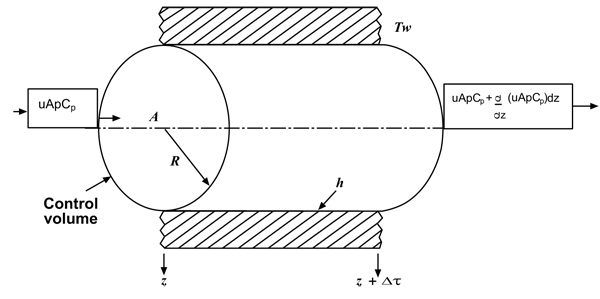 ).
).
 |
Fig. (1) Elemental or control volume for plug flow model. |
We act upon this elemental volume, which spans the whole of the tube cross section, with this general conservation law:
 |
(1) |
Since steady state is stipulated, the accumulation of heat is zero. Moreover, there are no chemical, nuclear, or electrical sources specified within the volume element, so heat generation is absent. The only way heat can be exchanged in this system is through the perimeter of the element by way of the temperature difference between wall and fluid.
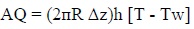
The incremental rate of heat removal were expressed as a positive quantity using Newton's law of cooling, that is,
 |
(2) |
As a convention, we expressed all such rate laws as positive quantities, invoking positive or negative signs as required for the expressions in conservation law (Eq. 1). The contact area in this simple model is simply the perimeter of the element multiply by its length. The constant heat transfer coefficient is denoted by h.
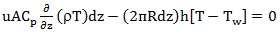
Now, along the axis, heat can enter and leave the element only by convection flow, so we can write the elemental form of Eq. 1 as:
 |
(3) |
(Rate heat flow in) (Rate heat flow out) (Rate heat loss through wall)
The first two terms are simply mass flow rate multiplied by local enthalpy, where the reference temperature for enthalpy is taken as zero. If Cp(T — Tref) was used for enthalpy, the term Tref will be cancelled in the elemental balance.
Simplifying then yields the sought-after differential equation
 |
(4) |
Where the negative signs have been cancelled.
Before solving this equation, it is good practice to group parameters into a single term (lumping parameters). For such elementary problems, it is convenient to lump parameters with the lowest order term as follows:
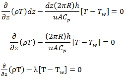 |
(4b) |
Where 
However, to solve the above equation requires a functional relationship between T and ρ for the gas, which were derived from the general gas law to be:
 |
(5) |
Showing the inverse relationship between temperature and density for gases where:
Mw = molecular weight of the gas stream and z = the compressibility factor.
Numerous Equations of State (EOS) models have been developed. Suffice it to say that polynomial equations that are cubic in molar volume offer the best compromise of accurately describing the behavior of fluids over wide range of operating conditions. They include: Van der Waal, Redlich-Kwong (RK), Soave-Redlich-Kwong (SRK), and Peng-Robinson (PR), equation of states. SRK and PR EOS have been found to provide results sufficiently accurate for engineering purposes, they are given below:
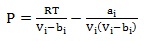 |
(6) |
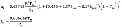
Where the EOS parameters, ai and bi are given for each model as follows:
For SRK:
 |
(7) |
For PR:
 |
(8) |
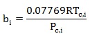 |
(9) |
Where
Tc, I is the critical temperature of component i
Pc,I is the critical pressure of component i
Tr, I is the reduced temperature of component i, Tr,I = Tc,i/T
wi is the accentric factor, which is actually the vapour pressure at 0.7Tr,i
Vapor viscosity is accurately correlated as a function of temperature by the relation:
 |
(10) |
Constants A, B, C, D for about 1500 compounds for both viscosities are available in the DIPPR (AIChE Design Institute for Physical Property Data).
However, for prediction of the vapor viscosity of pure hydrocarbons at low pressure (below Tref of 0.6), only the molecular weight, the critical temperature, and the critical pressure are required as follows:
µy = 4.60 × 10⁻⁴ NM1/2 Pc2/3/Tc1/2
N = 0.0003400Te004 for Tc ≤ 1.5
 |
(11) |
The resultant viscosity is in centipoises (mPa·sec), if Tc and Pc are given in K and Pa, respectively.
Thus, because of the implicit relationships in the above equations, their evaluation involves iterative techniques via software.
3.1. Heat Transfer in Pipelines
The basic equation for the analysis of heat conduction is Fourier’s law, which was based on experimental observations and is
 |
(12) |
Where the heat flux qn (W/m2) is the heat transfer rate in the n direction per unit area perpendicular to the direction of heat flow. kn(W/m · K) is the thermal conductivity in the direction n, and ∂T /∂n (K/m) is the temperature gradient in the direction n.
Thus the general equation of heat conduction in pipe (cylindrical coordinate system) was derived by performing an energy balance in conjunction with Fourier’s law:
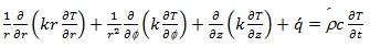 |
(13) |
3.1.1. Application
Fig. (2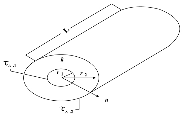 ) showed a hollow pipe of inside radius r1, outside radius r2, length L, and thermal conductivity k. The inside and outside surfaces are maintained at constant temperatures Ts,1 and Ts,2, respectively with Ts,1 > Ts,2 for steady-state conduction.
 |
Fig. (2) Radial conduction through a hollow cylinder. |
 |
(14) |
In the radial direction with no internal heat generation and constant thermal conductivity, the appropriate form of the general heat conduction equation, eq. (13), is
With the boundary conditions expressed as:
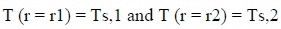 |
(15) |
3.1.2. Thermal Resistance
Thermal resistance is defined as the ratio of the temperature difference to the associated rate of heat transfer. This is completely analogous to electrical resistance, which, according to Ohm’s law, is defined as the ratio of the voltage difference to the current flow.
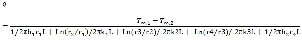
The rate of heat transfer q in a composite pipe is given by
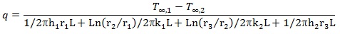 |
(16) |
Note that without insulation, eq. 17 reduces to:
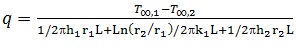 |
(17) |
Also for this case, where there is coating to prevent corrosion, equations 17 and 18 become:
 |
(18) |
 |
(19) |
3.2. Simulation
Thus using the above equations, one will simulate the system to predict the following:
- Temperature profile for insulated (normal operation) system
- Temperature profile for a failed insulation system
This involved numerical techniques. For these purposes the pipe is divided into grids or Sections ∆Z= Zi – Zi-1 as shown in figure below:
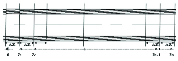 |
Modelling the system, the total heat loss for the entire pipe in each case from the exit temperature were computed from the formula:
 |
(20) |
Where M = mass flow rate of the gas = ρuA
Total heat loss for the pipeline, Q is found as the summation of heat losses in each segment, Qi
Thus,

For the normal operation (without insulation failure) Qi was found by calculating for each segment as follows
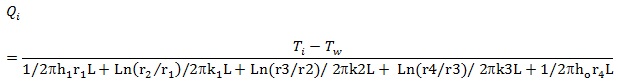 |
(21) |
The computed outlet temperature was compared with the operating value. Once the model predicts the operating value of the exit temperature, (at least within statistical level of significance) then a plot of Ti vs Zi was made to give the temperature profile for normal operation. Then, the model was deployed for the more rigorous analysis for failed system as shown below:
In this category, insulation failure in each segment (grid) were considered with the assumption that insulation failure implies insulation thickness, x = 0. For insulation failure in the 1st segment, the diagram is as follows:
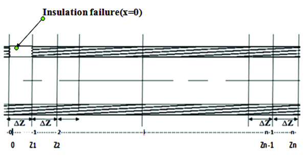 |
As previously shown, the total heat loss (from where the exit temperature is evaluated) is the summation of the heat losses in each segment, with the segment where insulation failure occurred evaluated. Equation 22 was adopted in this case as:
 |
(22) |
While all the other segments without insulation failure were evaluated using equation 21.
4. RESULTS AND DISCUSSION
The study model was validated using the field data in Table 1 and the length of the pipe under consideration is 55 kilometers.

Using the data in conjunction with the above model equations 1 to 10, temperature profiles has been calculated using a software, while the heat losses and the corresponding exit gas temperatures, for normal and insulation failure at different pipe length were calculated using equations 11 to 23.
Model Validation
The model was validated using field data as shown in Fig. (3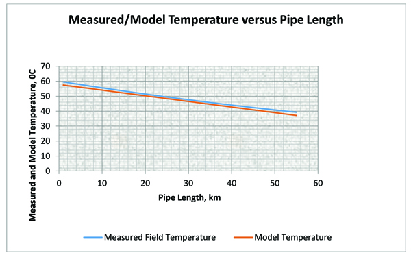 ). Actual field temperature and that calculated using the model was presented in a plotted and compared. The close match shows that the model can predict the temperature distribution of an insulated gas pipeline.
 |
Fig. (3) A plot of Measured and Model temperature and Pipe Length. |
From the Fig. (4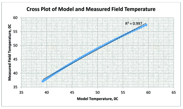 ), it is observed that the model can predict the temperature distribution in normal operation of a gas pipeline. The cross plot shows an R-Factor of 0.997 confirming the accuracy of the model.
 |
Fig. (4) A cross plot of Field Temperature Data and Model Temperatures Data. |
5. DISCUSSION
Considering a pipeline system of 55 km, Table 2 gives the temperature and pressure distribution along the whole length of the pipe while Fig. (5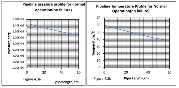 ) is the corresponding plot showing the temperature and pressure profiles along the pipe line. It can be observed that temperature and pressure decrease along the pipe line owing to frictional resistances to the flow.

 |
Fig. (5) A plot of Temperature versus Pipe Length. |
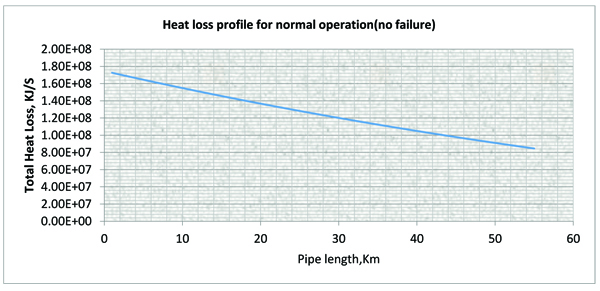 |
Fig. (6) A Plot of Total Heat Loss versus Pipe Length. |
Table 3 gives the total energy loss for a normal operation (without insulation failure) while Fig. (6 ) is the corresponding total heat loss profile.

This is because the Total heat loss is a direct function of the difference between the inlet temperature and the pipe wall temperature. The higher the difference, the more heat loss along the pipe.
Table 4 gives the total energy loss for a failed insulation while Fig. (7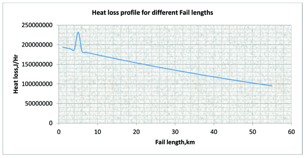 ) is the corresponding total energy loss with pipe length.

 |
Fig. (7) Heat loss versus distance of insulation failure (insulation failed between 4 -6km) |
This shows that the heat loss will increase when the insulation fails Table 5. This is as a result of inverse relationship between total heat loss and thermal resistance Fig. (8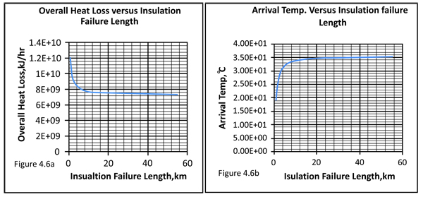 ) (Insulation failure implies reduction in thermal resistance).

 |
Fig. (8) A plot of Overall Heat Loss versus Insulation failure Length. |

It can be deduced from Fig. (9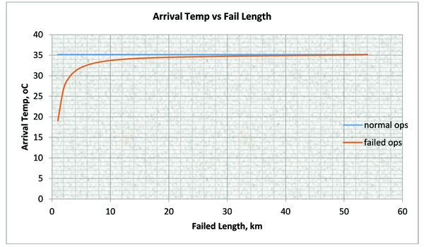 ), that the arrival temperature is constant for normal operation (that is when there is no insulation failure) because the overall heat loss is constant but the arrival temperatures varies (reduces) for failed operations due to increase in the overall heat loss resulting from the reduction in thermal resistance at the pipe section where the insulation failed. The reduction in arrival temperature is pronounce when the insulation failure is closer to departure point due to high heat loss at that point and approaches the value of that of normal operation when the failure is close to the arrival point due to low heat loss at that point.
 |
Fig. (9) A plot of Arrival Temperature versus pipe length for Normal and Insulation Failed length. |
CONCLUSION
In this study, it has been shown that in gas pipeline flow, exit temperature increases exponentially with the distance of insulation failure, and approaches the normal operation if the failure occurs towards the exit of the pipe.
A predictive model that predicts insulation failure and the pipeline location where it occurred was also developed. Thus, by merely reading the exit temperature, one will not only ascertain if insulation failure has occurred, but will also know the location of the pipe where it has occurred, so that remedial measures will be promptly taken without waste of time and resources searching for the location.
In this study, we have observed the following points in the subsea gas pipeline flow:
- The exit temperature increases exponentially with the distance of insulation failure, and approaches the normal operation if the failure occurs towards the exit of the pipe.
- A predictive model that predicts insulation failure and the pipeline location where it occurred was proposed and developed.
- Like all numerical techniques, the smaller the grid size, the better the results, but with increased rigour.
- The model developed can be used to check the readings of an optic-fibre distributed temperature sensors.
- After developing this model using classical visual basic and excel package, the model was validated by cross plotting the normal temperature profiles of the model and field data; and R-factor of 0.997 was obtained.
- Analysis of the results from the model showed that insulation failure can be predicted on a real time basis.
CONSENT FOR PUBLICATION
Declared none.
CONFLICT OF INTEREST
The authors declare no conflict of interest, financial or otherwise.
ACKNOWLEDGEMENTS
Declared none
REFERENCES
| [1] | M. Roche, D. Melot, and G. Paugam, "Recent experience with pipeline coating failures", In: 16th International Conference on Pipeline Protection, BHR Group, 2-4 November, Paphos, Cyprus, 2005. |
| [2] | C. Melve, A. Rydin, and B. Hansen, "Long term testing of high temperature thermal insulation for subsea flow lines at simulated seabed conditions", 15th International Conference on Pipeline Protection, . |
| [3] | M. Batallas, and P. Singh, "Evaluation of Anticorrosion Coatings for High Temperature Service", NACE Corrosion, paper no. 08039, . |
| [4] | B. Hansen, and C. Rydin, Development and Qualification of Novel Thermal Insulation Systems for Deepwater Flowlines and Risers based on Polypropylene.OTC 2002, paper no. 14121 Houston., OTC: TX, . [http://dx.doi.org/10.4043/14121-MS] |
| [5] | J.A. Beavers, Thompson NG. External corrosion of oil and natural gas pipelines. ASM handbook. 2006;13:1015-25. |
| [6] | D.R. Dott, Optimal Network Design for Natural Gas Pipelines., University of Calgary: Alberta, pp. 57-90.http://dspace.ucalgary.ca/bitstream/1880/ 26992/1/31387Dott.pdf |
| [7] | B. Douglas, D. Pugh, C. Monahan, and P. Russ, "Top of Line Corrosion Management through Innovative Subsea Facility Design", International Petroleum Technology Conference, . [http://dx.doi.org/10.2523/IPTC-12788-MS] |
| [8] | Turner and Malloy, Handbook of Thermal Insulation Design Economics for Pipes and Equipment., Krieger: New York, . |
| [9] | M. Aggour, Petroleum Economics and Engineering, edited by Abdel- Aal, H. K., Bakr, B. A., and Al-Sahlawi, M., Marcel Dekker, Inc., p. 309. |
| [10] | ETI- Economic Thickness for Industrial Insulation, Conservation Pap. 46, Federal Energy Administration, August 1976 Piping Insulation-Economics and Profits vol.69, 1982, pp. 27–46. |
| [11] | R.H. Paul, "Common law and statute law", J. Legal Stud., vol. 11, no. 2, pp. 205-223. [http://dx.doi.org/10.1086/467698] |
| [12] | B. Guo, S. Duan, and A. Ghalambor, "A simple model for predicting Heat loss and Temperature profiles in Insulated pipelines", SPE Prod. Oper., vol. 21, no. 1, pp. 107-113. [http://dx.doi.org/10.2118/86983-PA] |
| [13] | M.M. Salama, "An alternative to api 14e erosional velocity limits for sand-laden fluids", J. Energy Resour. Technol., vol. 122, no. 2, p. 71. [http://dx.doi.org/10.1115/1.483167] |
| [14] | B.S. McLaury, and S.A. Shirazi, "An alternative method to api rp 14e for predicting solids erosion in multiphase flow", J. of Energy Resources Techno., Transac. of the ASME, vol. 122, no. 3, pp. 115-122. [http://dx.doi.org/10.1115/1.1288209] |
| [15] | Q.H. Mazumder, S.A. Shirazi, B.S. McLaury, J.R. Shadley, and E.F. Rybicki, A mechanistic model to predict erosion in multiphase flow in elbows downstream of vertical pipes, 2004. |