- Home
- About Journals
-
Information for Authors/ReviewersEditorial Policies
Publication Fee
Publication Cycle - Process Flowchart
Online Manuscript Submission and Tracking System
Publishing Ethics and Rectitude
Authorship
Author Benefits
Reviewer Guidelines
Guest Editor Guidelines
Peer Review Workflow
Quick Track Option
Copyediting Services
Bentham Open Membership
Bentham Open Advisory Board
Archiving Policies
Fabricating and Stating False Information
Post Publication Discussions and Corrections
Editorial Management
Advertise With Us
Funding Agencies
Rate List
Kudos
General FAQs
Special Fee Waivers and Discounts
- Contact
- Help
- About Us
- Search


The Open Atmospheric Science Journal
(Discontinued)
ISSN: 1874-2823 ― Volume 14, 2020
A Synoptic Study of Low Troposphere Wind at the Israeli Coast
Sigalit Berkovic1, 2, *, Pinhas Alpert2
Abstract
Objective:
This research is dedicated to the study of the feasibility of surface wind downscaling from 925 or 850 hPa winds according to synoptic class, season and hour.
Methods:
Two aspects are examined: low tropospheric wind veering and wind speed correlation and verification of the ERA-Interim analysis wind by comparison to radiosonde data at Beit Dagan, a station on the Israeli coast.
Results:
Relatively small (< 60°) cross angles between the 1000 hPa wind vector and the 925 hPa or 850 hPa wind vector at 12Z and high correlation (0.6-0.8) between the wind speed at the two levels were found only under winter lows. Relatively small cross angles and small wind speed correlation were found under highs to the west and Persian troughs.
The verification of ERA-Interim analysis in comparison with radiosonde data has shown good prediction of wind direction at 12Z at 1000, 925 and 850 hPa levels (RMSE 20°-60°) and lower prediction quality at 1000 hPa at 0Z (RMSE 60°-90°). The analysis under-predicts the wind speed, especially at 1000 hPa. The wind speed RMSE is 1-2 m/s, except for winter lows with 2-3 m/s RMSE at 0Z, 12Z at all levels.
Conclusion:
Inference of surface wind may be possible at 12Z from 925 or 825 hPa winds under winter lows. Inference of wind direction from 925 hPa winds may be possible under highs to the west and Persian troughs. Wind speed should be inferred by interpolation, according to historical data of measurements or high resolution model.
Article Information

Identifiers and Pagination:
Year: 2018Volume: 12
First Page: 80
Last Page: 106
Publisher Id: TOASCJ-12-80
DOI: 10.2174/1874282301812010080
Article History:
Received Date: 1/4/2018Revision Received Date: 17/7/2018
Acceptance Date: 23/7/2018
Electronic publication date: 13/08/2018
Collection year: 2018
open-access license: This is an open access article distributed under the terms of the Creative Commons Attribution 4.0 International Public License (CC-BY 4.0), a copy of which is available at: https://creativecommons.org/licenses/by/4.0/legalcode. This license permits unrestricted use, distribution, and reproduction in any medium, provided the original author and source are credited.
* Address correspondence to this author at Department of Mathematics, Israel Institute for Biological Research, Ness Ziona, Israel; Tel: 972-8-938-1656; E-mail: sigalitb@iibr.gov.il
| Open Peer Review Details | |||
|---|---|---|---|
| Manuscript submitted on 1-4-2018 |
Original Manuscript | A Synoptic Study of Low Troposphere Wind at the Israeli Coast | |
1. INTRODUCTION
Deep winter cyclones over the Eastern Mediterranean are accompanied by extreme western wind events over Israel e.g [1Navarra A, Tubiana L. Regional Assessment of Climate Change in the Mediterranean 2013., 2Lionello P. The clime of the Mediterranean Region 2012.]. A critical effect of these extreme winds is the erosion of the coastline and the need for civil authorities to prepare for this challenge [3Kit K. Marine Policy Plan for Israel 2014.http:// msp-israel.net.technion.ac.il /files/2014 /12/ATOS-report -final.pdf-5Herrmann M, Somot S, Calmanti S, Dubois C, Sevault F. Representation of spatial and temporal variability of daily wind speed and of intense wind events over the Mediterranean Sea using dynamical downscaling: Impact of the regional climate model configuration. Nat Hazards Earth Syst Sci 2011; 11: 1983-2001.
[http://dx.doi.org/10.5194/nhess-11-1983-2011] ]. A possible way is to use weather models; however, this effort demands extensive resources. Hence, statistical downscaling of extreme surface wind events is needed. Global climate models often underestimate the wind at 1000 hPa [5Herrmann M, Somot S, Calmanti S, Dubois C, Sevault F. Representation of spatial and temporal variability of daily wind speed and of intense wind events over the Mediterranean Sea using dynamical downscaling: Impact of the regional climate model configuration. Nat Hazards Earth Syst Sci 2011; 11: 1983-2001.
[http://dx.doi.org/10.5194/nhess-11-1983-2011] -7Lavaysse C, Vrac M, Drobinski P, Lengaigne M, Vischel T. Statistical downscaling of the french mediterranean climate: Assessment for present and projection in an anthropogenic scenario. Nat Hazards Earth Syst Sci 2012; 12: 651-70.
[http://dx.doi.org/10.5194/nhess-12-651-2012] ], and sometimes the 1000 hPa is not available [8Hochman A, Harpaz T, Saaroni H, Alpert P. Synoptic classification in 21st Century CMIP5 predictions over the Eastern Mediterranean with focus on cyclones, accepted for publication Int. J Clim 2017.]. Hence, the ability to infer surface winds from low troposphere data should be considered. This work examines the feasibility to employ data from low troposphere climate models in order to statistically downscale wind according to the semi objective synoptic classification.
The definition of the semi objective synoptic classes [9Alpert P, Osetinsky I, Ziv B, Shafir H. Semi-objective classification for daily synoptic systems: Application to the Eastern Mediterranean climate change. Intern J Climatol 2004; 24: 1001-11.http:// www.tau.ac.il/ ~pinhas/papers/2004 /Alpert_et_al _IJC_2004a.pdf, 10Osetinsky I. Climate changes over the E. Mediterranean-A synoptic systems classification approach. Ph.D. thesis, Tel Aviv University, 2006: 153 pp.] according to General Circulation Models (GCM) data [8Hochman A, Harpaz T, Saaroni H, Alpert P. Synoptic classification in 21st Century CMIP5 predictions over the Eastern Mediterranean with focus on cyclones, accepted for publication Int. J Clim 2017.] and the relation between synoptic classes and historical measured surface winds will enable the classification of future surface wind fields up to the next century. Furthermore, under winter lows over Israel, the ability to directly infer from low troposphere wind data suggests a simple alternative to downscaling extreme western wind events according to the semi objective synoptic classification.
The ability to use the semi objective synoptic class [9Alpert P, Osetinsky I, Ziv B, Shafir H. Semi-objective classification for daily synoptic systems: Application to the Eastern Mediterranean climate change. Intern J Climatol 2004; 24: 1001-11.http:// www.tau.ac.il/ ~pinhas/papers/2004 /Alpert_et_al _IJC_2004a.pdf] as a predictor for hourly surface wind along the central and the southern Israeli coast has been demonstrated [11Berkovic S. Synoptic classes as a predictor of hourly surface wind regimes: The case of the central and southern israeli coastal plains. J App Met Climatol 2016; 55(7): 1533 2016; 55(7): 1533. http://dx.doi.org/10.1175/JAMC-D-16-0093.1]. This approach is based on the idea that a given circulation pattern is often associated with similar local-scale meteorological conditions e.g. [12Zorita E, von Storch H. The analog method as a simple down-scaling technique: Comparison with more complicated methods. J Clim 1999; 12: 2474-89.
[http://dx.doi.org/10.1175/1520-0442(1999)012<2474:TAMAAS>2.0.CO;2] , 13Huth R. Disaggregating climatic trends by classification of circulation patterns. Int J Climatol 2001; 21: 135-53.
[http://dx.doi.org/10.1002/joc.605] ]. The current study extends [11Berkovic S. Synoptic classes as a predictor of hourly surface wind regimes: The case of the central and southern israeli coastal plains. J App Met Climatol 2016; 55(7): 1533 2016; 55(7): 1533. http://dx.doi.org/10.1175/JAMC-D-16-0093.1] in order to check whether it is possible to infer surface winds along the Israeli coast from high level winds (850 or 925 hPa) under the various semi objective synoptic classes and seasons at 0, 12Z. For this purpose, the horizontal wind turning at the low troposphere levels is examined. The study is limited to Beit Dagan, a representative station near the homogeneous central Israeli coastline (Fig. 1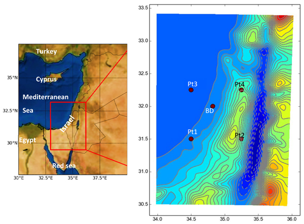 ). The limitation to a single station is derived from the fact that radiosonde data are scarce, and only available for this station.

The most prevalent geostrophic wind over the east Mediterranean has a westerly component [10Osetinsky I. Climate changes over the E. Mediterranean-A synoptic systems classification approach. Ph.D. thesis, Tel Aviv University, 2006: 153 pp.]. The sea breeze and upslope winds (Fig. 1), blowing from the sea to the land, during daytime have a westerly component, while the land breeze and downslope winds have an easterly component. At 12Z the mesoscale and the synoptic winds have similar directions (W component winds), therefore, the possibility to infer surface wind from higher level wind is expected to be successful. During the night hours the meso wind direction usually opposes the synoptic wind direction [11Berkovic S. Synoptic classes as a predictor of hourly surface wind regimes: The case of the central and southern israeli coastal plains. J App Met Climatol 2016; 55(7): 1533 2016; 55(7): 1533. http://dx.doi.org/10.1175/JAMC-D-16-0093.1, 14Berkovic S. Winter wind regimes over Israel using self-organizing maps. J Appl Meteorol Climatol 2017; 56: 2671-91.
[http://dx.doi.org/10.1175/JAMC-D-16-0381.1] , 15Skibin D, Hod A. Subjective analysis of mesoscale flow patterns in northern Israel. J Appl Meteorol 1979; 18: 329-38.
[http://dx.doi.org/10.1175/1520-0450(1979)018<0329:SAOMFP>2.0.CO;2] ] and a study of the Cross Angle (CA) at 0Z will reveal the relation between the surface wind and 925 or 850 hPa winds at this hour.
The boundary layer height over Israel is 1- 2 km [16Dayan U, Shenhav R, Graber M. The spatial and temporal behavior of the mixed layer in Israel. J Appl Meteorol 1988; 27: 1382-94.
[http://dx.doi.org/10.1175/1520-0450(1988)027<1382:TSATBO>2.0.CO;2] ]. Accordingly, the 925 hPa (~ 800 m) level is around or lower than the mixing layer height, while the 850 hPa (~1.5 km) level is mostly above the mixing height. Zaiter and Al-Jumaily [17Zaiter DS, Al-Jumaily KJ. Characteristics of thermal wind over iraq. Inter J Sci Res Publ 2016; 6: 163-7.] showed that the wind at 900-850 hPa at latitude 32º N, longitude 30º -50º E obeys the thermal wind equation according to NCEP data. We assume similar behavior according to ERA-Interim data. The ability to use reanalysis data was verified by comparing measurements to ERA-Interim data at the three levels according to season, hour and synoptic class. To the best of our knowledge, no such extensive quantitative verification has been made previously for our area. This verification gives an indication of the ability to use model data to infer the surface wind from low troposphere levels along the Israeli coast.
Section 2 will describe the method and data used in this study, section 3 will briefly describe the synoptic classes, and sections 4-6 will display the results of the CA histograms and verify ERA-Interim wind prediction. Summary and conclusions follow in sections 7 and 8.
2. METHODS AND DATA
Time series of radiosonde data over Israel are scarce and limited to Beit Dagan (BD), a station on the Israeli coastal plain with relatively flat topography. Therefore, the study is limited to this location at the hours 0, 12Z. BD radiosonde data at 0, 12Z at the 1000, 925 and 850 hPa pressure levels from the years 1974-2012 was downloaded from weather.uwyo.edu [18 weather.uwyo.edu weather.uwyo.edu http ://weather.uwyo.edu/ upperair/]. The available variables of the radiosonde data are: pressure, height, temperature, humidity and wind. Wind speeds were archived in full knots, therefore after converting into m/sec units the wind speed uncertainty is ±0.25 m/s.
A dataset of the synoptic classification for the investigated location and time period has been performed by our research group members according to the published synoptic classification of Alpert et al. [9Alpert P, Osetinsky I, Ziv B, Shafir H. Semi-objective classification for daily synoptic systems: Application to the Eastern Mediterranean climate change. Intern J Climatol 2004; 24: 1001-11.http:// www.tau.ac.il/ ~pinhas/papers/2004 /Alpert_et_al _IJC_2004a.pdf] and Osetinsky [10Osetinsky I. Climate changes over the E. Mediterranean-A synoptic systems classification approach. Ph.D. thesis, Tel Aviv University, 2006: 153 pp.].
The relation between synoptic classes and surface winds was previously defined [11Berkovic S. Synoptic classes as a predictor of hourly surface wind regimes: The case of the central and southern israeli coastal plains. J App Met Climatol 2016; 55(7): 1533 2016; 55(7): 1533. http://dx.doi.org/10.1175/JAMC-D-16-0093.1]. This has led us to a further study to investigate whether the 1000 hPa wind can be inferred from the 925 or 850 hPa wind according to synoptic class and season at each hour (12Z or 0Z). The surface pressure at BD is mostly 1000 -1010 hPa, and therefore 1000hPa wind is very similar to the surface wind.
The synoptic classification is the semi–objective classification derived by Alpert et al. [9Alpert P, Osetinsky I, Ziv B, Shafir H. Semi-objective classification for daily synoptic systems: Application to the Eastern Mediterranean climate change. Intern J Climatol 2004; 24: 1001-11.http:// www.tau.ac.il/ ~pinhas/papers/2004 /Alpert_et_al _IJC_2004a.pdf] determined according to temperature, geopotential, and horizontal wind components at 1000 hPa over the East Mediterranean (EM) from NCEP/NCAR data. The frequent synoptic classes, presented in Table 1, were selected in order to ensure a large number of instances (> 30) under each season and synoptic class at each hour. A description of the synoptic classes is given in the following section.

In order to study the low troposphere winds along the Israeli coast, the following methodology was performed:
Firstly, the wind turning was studied according to the Cross Angle (CA) between the wind vectors of the two levels 1000, 925 hPa or 1000, 850 hPa (abbreviated as CA925, CA850). The CA is the angle created due to the subtraction of the lower level wind vector from the upper level wind vector. The wind may be veering or backing (clockwise or counterclockwise), therefore, the sign of the turning is kept and designated by + or – respectively. This definition is after the well-known thermal wind relationship between geostrophic wind direction vertical shear and horizontal temperature advection [19Holton JR. An Introduction to Dynamic Meteorology 4th ed. 2004.-23Wang S, O’Neill LW, Jiang Q, et al. A regional real time forecast of marine boundary layers during VOCALS-Rex. Atmos Chem Phys 2011; 11: 421-37.
[http://dx.doi.org/10.5194/acp-11-421-2011] ]. Since wind direction can be determined meaningfully only when the wind speed is higher than 0.5 m/s, CA925 or CA850 was calculated if the wind speed at the two relevant levels were greater than 0.5 m/s. In order to facilitate the verification of wind direction uniformity at two levels a small CA criterion has been set. A previous study of surface wind steadiness along the Israeli coast according to synoptic class [11Berkovic S. Synoptic classes as a predictor of hourly surface wind regimes: The case of the central and southern israeli coastal plains. J App Met Climatol 2016; 55(7): 1533 2016; 55(7): 1533. http://dx.doi.org/10.1175/JAMC-D-16-0093.1] has shown that a high degree of wind steadiness is obtained under winter lows, and then the standard deviation of the wind direction is ~ 60°. Therefore, our criterion for a small CA (SC) value is the % of events bounded by 60°. The maximal CA in this study is 180º. Under all the studied events, the pressure at the station-level was equal to, or greater than 1000 hPa (1000-1027 hPa).
The correlation between the wind speed at the two levels 1000, 925 hPa or 1000, 850 hPa was verified according to scatter plots (not shown) and the Pearson correlation was calculated (python software pearsonr function from scipy.org [24 Scipy.org https:// docs.scipy.org /doc/scipy -0.14.0/reference /generated/ scipy.stats.pearsonr.html]). The Pearson correlation coefficient measures the linear relationship between two data sets and requires that each dataset be normally distributed.
Secondly, a comparison between ECMWF (European Centre for Medium-Range Weather Forecasts) ERA-Interim (European Reanalysis) analyzed wind [25Apps.ecmwf.int. ERA Interim, Daily. [online] 2017. Available at:
http:// apps.ecmwf.int/ datasets/data /interim-full- daily/, 26Berrisford P, Dee DP, Poli P, et al. The ERA-interim archive version 2.0 2011.
Available from: http:// www.ecmwf.int/ en/elibrary/ 8174-era-interim -archive-version-20] and the radiosonde data was performed by bilinear interpolation of data at the grid points closest to BD at each pressure level. The native model resolution is ~ 80 km. The downloaded interpolated data horizontal resolution is 0.75° (~ 83 km). (Fig. 1) displays the location of BD and its closest ERA-Interim grid points. Point3 (Pt3) is over the Mediterranean Sea, point1 (Pt1) is on the seashore as is BD, point4 (Pt4) and point2 (Pt2) are inland points over complex topography. The terrain height at BD (lat 32.0073, lon 34.8138) is 31m ASL. The Samaria and Judea mountains run north to south, east of BD. The peak height is 400 meters above sea level.
The comparison of ERA-Interim vs. BD radiosonde horizontal wind at 1000, 925 and 850 hPa was performed firstly according to seasons and hours, and secondly according to seasons, synoptic classes and hours. Scatter plots of wind speed and direction presenting measurements versus reanalysis values were drawn; however, they are too numerous to be shown. The statistical parameters that were derived from the scatter plots - bias, RMSE, correlation and the linear interpolation slope (a) and intercept (b) - will be summarized and presented. For the second comparison which included the synoptic classes only RMSE will be presented.
3. EM SYNOPTIC GROUPS AND CLASSES
This description of synoptic groups and classes was given in [9Alpert P, Osetinsky I, Ziv B, Shafir H. Semi-objective classification for daily synoptic systems: Application to the Eastern Mediterranean climate change. Intern J Climatol 2004; 24: 1001-11.http:// www.tau.ac.il/ ~pinhas/papers/2004 /Alpert_et_al _IJC_2004a.pdf-11Berkovic S. Synoptic classes as a predictor of hourly surface wind regimes: The case of the central and southern israeli coastal plains. J App Met Climatol 2016; 55(7): 1533 2016; 55(7): 1533. http://dx.doi.org/10.1175/JAMC-D-16-0093.1] and is briefly repeated here for the benefit of the reader. Table 1 summarizes the main 4 groups and their classes. Full presentation of the synoptic classes is given in Fig. (2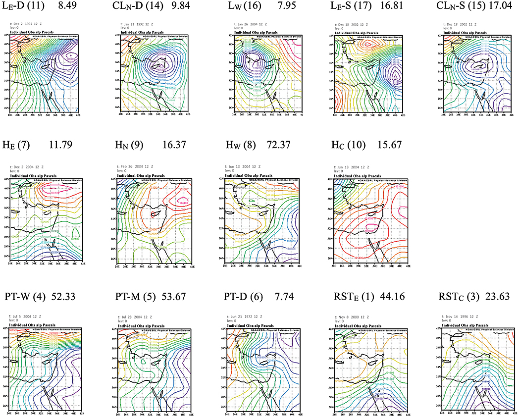 ) [11Berkovic S. Synoptic classes as a predictor of hourly surface wind regimes: The case of the central and southern israeli coastal plains. J App Met Climatol 2016; 55(7): 1533 2016; 55(7): 1533. http://dx.doi.org/10.1175/JAMC-D-16-0093.1].
There are two main seasons in the EM-the dry season in summer (mid-June–September) and the wet season in winter (December–February)-as well as the “transition months” (April–May, October–November). Five synoptic groups characterize this climate. A single group is dominant during the summer, and four groups prevail during the winter and the transition months. The fifth group “sharav lows” is rare and was not included in our study.
1. The Persian trough – abbreviated PT-is a persistent synoptic class during the summer months (mid-June–September). This trough extends from the Asian monsoon through the Persian Gulf along southern Turkey and the Aegean Sea. The depth of the PT changes during the summer. Deep troughs reach Greece while shallow troughs do not reach the Mediterranean Sea. There is practically no rain during the summer. Since the synoptic situation is static, a remarkable daily periodicity is obtained in the EM during the summer. The flow over the area is mainly determined by mesoscale and microscale processes. Northwesterly synoptic winds flow over the EM as a result of the PT and the NW Etesian winds. During early morning hours, when the temperature gradient between air and sea is minimal, the synoptic wind is mostly W-SW.
2. The winter Lows (Ls) and Cyprus Lows (CLs) form the dominant synoptic group during winter (Fig. 2, first row). They are responsible for the largest amount of rain in the EM. CLs are the main contribution to the winter lows, each contributing rainfall during two to three consecutive days. The name CL is given to Mediterranean cyclones that reach the EM; they need not be located over Cyprus itself to be designated CLs. Deep lows are characterized by strong (max ~10 m/s) westerly winds.
3. Highs:
a) The “Siberian highs” (winter highs) occur mainly during the cool season. Siberian highs are highs of a northern origin: Europe (e.g., Romania, Turkey and Caucasia) or Siberia (the winter Asiatic monsoon) itself. The extension of the Siberian high is rare, occurring once every few years. It is accompanied by cold, dry northeasterly winds that last for several days. Winter highs bring fair weather, inducing cold, dry northerly to easterly winds over Israel.
b) The “subtropical high” (the High to the west of Israel [HW]) may occur throughout the year. It is an extension of the Azores high, which prevails over North Africa. When this high is extended further to the east and reaches Israel, it brings NW winds with humid air from the sea.
4. The Red Sea Trough (RST), a trough over the Red Sea and its surroundings, is an extension of a low over the Sudan, which may occur during the transition months or during winter. It is characterized by a dry easterly flow east of the trough axis. When an upper trough stretches over the EM, the RST develops northward and deepens. As a result, rain clouds may develop. Convective storms may evolve and cause floods over southern Israel and Sinai, especially with ground heating during the day.
 |
Fig. (2) Typical examples for the EM frequent (more than 5 days/year) synoptic classes as defined by Alpert et al. 2004. Each map is a SLP (hPa) map from a representative day (Osetinsky 2006). The frequency of each synoptic class (number of days per year) is denoted above each SLP map. The winter lows are presented in the first row: Low east deep (LE-D), Deep Cyprus low from the north (CLN-D), cold low from the west (LW). Highs are presented in the second row: High from the north (HN), High from the west (HW) and high over Israel (HC). Troughs are presented in the third row: Medium Persian trough (PT-M), Red sea trough to the east (RSTE) and Red sea trough center (RSTc). The subfigures were downloaded from http:// www.esrl.noaa.gov/ psd/ data/ gridded/ data.ncep.reanalysis.html |
The fifth group “sharav lows” is rare and was not included in our study.
The subdivision of the four major synoptic groups provides the 14 most frequent classes referred to in this work. The divisions are made according to the location/depth and the field gradients of the classes over the EM region.
The CL group includes the following classes: The Deep CL to the north (CLN-D) and the Shallow CL to the north (CLN-S). The L group includes these classes: the Cold low to the west (LW), the Deep low to the east (LE-D) and the Shallow low to the east (LE-S).
The RST group includes these classes: the RST with an eastern axis (RSTE) and the RST with a central axis (RSTC). The location of the axis is defined relative to the EM coastline.
PTs are divided into three classes: deep, medium and shallow (respectively, PT-D, PT-M and PT-W). Siberian highs (winter highs) are divided into three classes: north, east and over Israel (respectively, HN, HE and HC). The summer subtropical high is known as HW. The names are based on the location of the pressure gradient.
4. RESULTS
4.1. CA at BD as a Function of Hour, Synoptic Class and Seasonality
The CA925 histograms were “squeezed” into bar and whiskers plots (boxplots) in order to present simultaneously the results for the most frequent synoptic classes according to seasons and hours (0Z or 12Z). These results are displayed in Fig. (3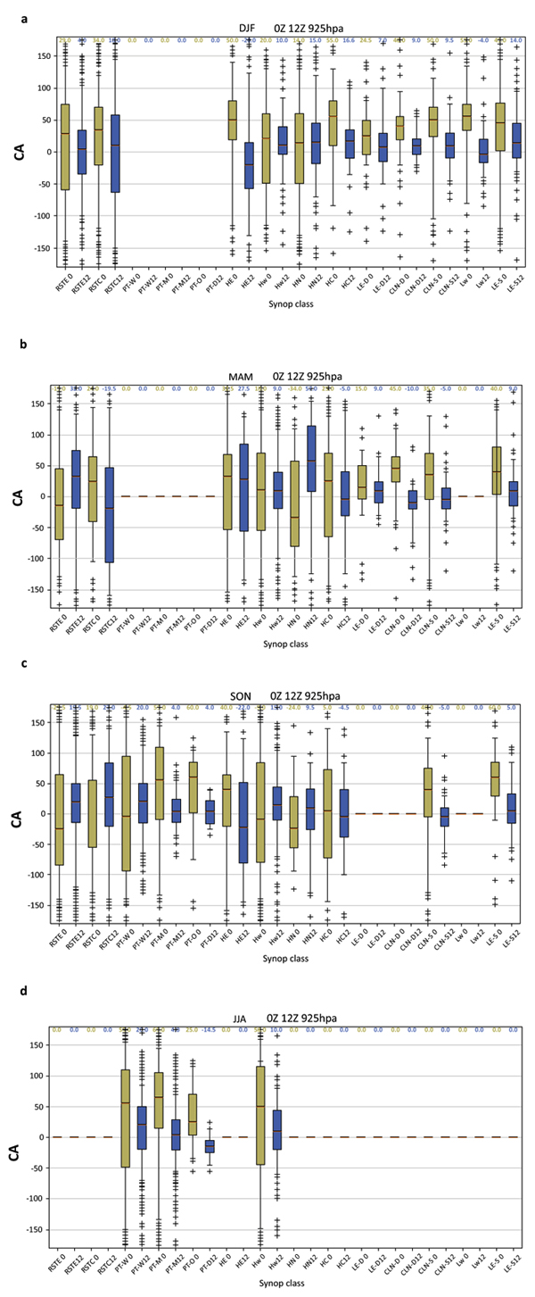 ) (a-DJF b-MAM c-SON d-JJA). The numbers of the events in each of the boxplots displayed in Fig. (3) are summarized in Table 2. Each box indicates the median and quartiles (25th and 75th percentiles). The whiskers display the 5th and 95th percentiles. (50% of the results are within each box, 90% of the results are within the whiskers). Table 3 summarizes the % of events bounded by 60°, which is our criterion for a small CA (SC) value, as the maximal CA in this study is 180º. Under the winter lows (LE-D CLN-D CLN-S LW LE-S, presented at the right 10 columns of the figures) at 12Z small CA925 (SC) values are found 77-93% of the time – (Table 3) PT’s and Hw also adhere to the SC criterion in 74-100% of the cases. These relatively small CA values result from the fact that the 925 hPa level is below the boundary layer height, when mostly neutral thermal stability is dominant.


The basic theory describing the flow in the boundary layer is the well-known Ekman model [18 weather.uwyo.edu weather.uwyo.edu http ://weather.uwyo.edu/ upperair/, 27Zhemin T, Juan F, Rongsheng W. Nonlinear Ekman layer theories and their applications. Acta Meteorol Sin 2006; 20: 209-22., 28Stull RB. Introduction to boundary layer meteorology 2003.] which addressed the Coriolis force, pressure gradient force and frictional force due to turbulence in the Boundary Layer (BL). This theory captures the main properties of the wind in the boundary layer. The horizontal wind speed increases with altitude and the wind vector veers with height (Ekman spiral). Near the surface the flow turns toward the low pressure. The ageostrophic flow next to the surface initiates convergence and creates vertical flow at the top of the BL (Ekman pumping). This pumping is the primary mechanism through which the entire atmosphere responds to the BL processes. The Ekman theory gives only a qualitative description due to the nonlinear and non-homogeneous nature of the BL flow. Many derivations of BL models were later developed [29Beljaars A. The parametrization of the planetary boundary layer 1992. Available from: https:// www.ecmwf.int /sites/ default/ files/elibrary/ 2002/16959-parametrization -planetary- boundary- layer.pdf, 30Plant B. Boundary Layer Parameterization 2014. Available from: http:// www.met.reading .ac.uk/~ sws00rsp/teaching /nanjing/blayer.pdf]. The thermal stability plays a crucial role in the features of the BL flow. It appears that stability could explain the major differences between the CAs at 12Z vs. 0Z.

The Ekman spiral theory, assuming neutral stratification and barotropic environment, predicts a CA of 45° between the surface and the top of Ekman layer. The Ekman layer height is usually below the 850 hPa level of ~ 1.5 km (e.g., eq. 5.26-7 in [18 weather.uwyo.edu
weather.uwyo.edu http ://weather.uwyo.edu/ upperair/], eq. 7.30 in [31Arya SP. Introduction to Micrometeorology 1988; 307.]). The well-mixed model - assuming constant mean potential temperature and constant wind profiles in the boundary layer - predicts CA~30°. According to measurements, the CA is 20° - 70° in baroclinic PBL and ~ 35° above neutral barotropic rough area ([29Beljaars A. The parametrization of the planetary boundary layer 1992.
Available from: https:// www.ecmwf.int /sites/ default/ files/elibrary/ 2002/16959-parametrization -planetary- boundary- layer.pdf], p.97, Ch. 6.3). At 0Z, this is not the case. The boundary layer height decreases to less than 1 km and stable thermal stability is dominant. Even under deep winter lows (CLN-D LE-D), the local easterly flow (land breeze and downslope wind) increases the CA925 (only 49-82% adhere to SC, Table 3). The spread of the histograms at 0Z is larger than the spread at 12Z for all seasons (Fig. 3), probably due to enhanced thermal stability during the night, indicating low correlation between the surface flow and the flow at the higher levels (925, 850 hPa). To summarize, only 12Z wind data can infer the wind direction at the surface.
CA850 histograms are similar to those presented for CA925 histograms in Fig. (3) The spread of the CA850 histograms is larger than the corresponding spread in Fig. (3) The CA increases with increasing distance between the two levels, as stated by the Ekman spiral theory. Due to similarity, these results are displayed in the supplementary material (Fig. S1 , Tables S1 and S2). The same conclusions are derived from the CA850 histograms. Under winter lows, 65-91% of the CA850 magnitudes at 12Z show SC, however, at 0Z only 35-68% do. Hw and PT-D have relatively high frequencies (49-70% and 85% respectively).
In order to verify the possibility of inferring extreme wind events, the above statistics were repeated only for these events. The speed of the upper 90% percentile at 925 and 850 hPa were calculated and their values are 7 and 8 m/s respectively. Figs. (4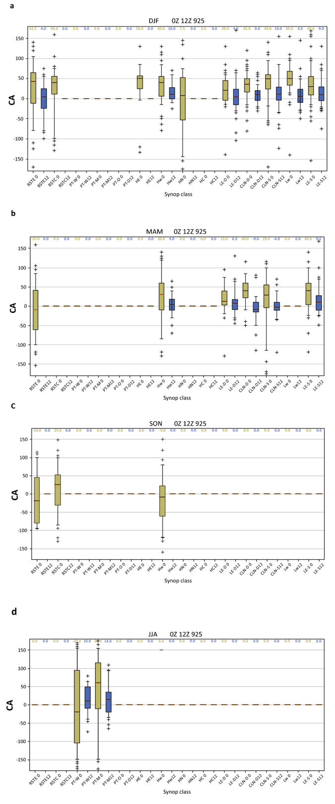 , 5
, 5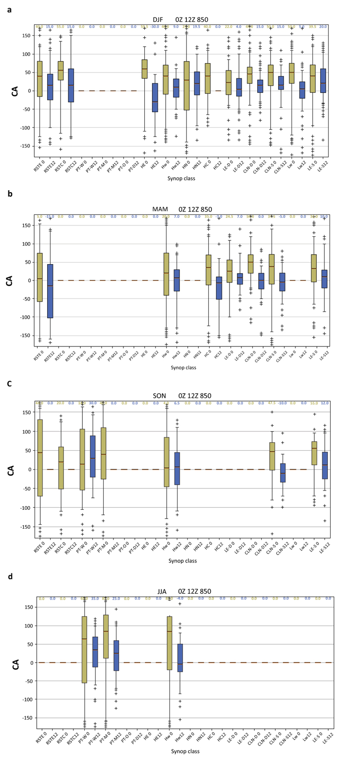 ) display boxplots of these events according to season, synoptic class and hour. Tables 4 and 6 summarize the number of events according to the boxplots presented in Figs. (4, 5) A comparison of Tables 4 and 2 shows higher frequency of strong wind events under the winter lows, as expected. Tables 5 and 7 present the % of events adhering to SC.

The number of the events of each CA925 boxplot displayed in Fig. (4
). Only extreme wind events at 925 hPa are included.


The number of CA850 events according to the boxplots in Fig. (5
). Only extreme wind events at 850 hPa are included.
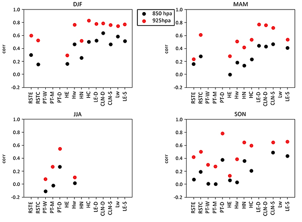 |
Fig. (6) The correlation between wind speed at 1000,925 hPa levels (red) and 1000,850 hPa levels (black) at 12Z. The correlation was calculated when more than 30 events were found. The number of events is displayed in Table 2 and Table S1. |
Under winter lows and Hw at 12Z, 79-100% of the CA925 exhibit SC, and therefore good inference of wind direction is achieved. Slightly smaller frequency, 72-100%, was found for the CA850 SC events under winter lows. At 0Z, on the other hand, only 60-88% of CA925 and 42-74% CA850 are SC. Extreme wind events under winter lows at 0Z still show relatively high CA values. Wider ranges of CA values under all the synoptic groups at 0Z might be related to the thermal stability. During the night hours stable conditions prevent efficient interaction between the vertical levels. The monthly average stable atmospheric boundary layer height is 400 ± 200 m and the frequency of events is 15-20 days per month during autumn and winter and 10-15 days per month during spring and summer [32Dayan U, Rodnizky J. The temporal behavior of the atmospheric boundary layer in Israel. J App Met 1999; 38: 830.
[http://dx.doi.org/10.1175/1520-0450(1999)038<0830:TTBOTA>2.0.CO;2] ]. During the daytime, the mixing layer height usually prevails between 1000 and 850 hPa [16Dayan U, Shenhav R, Graber M. The spatial and temporal behavior of the mixed layer in Israel. J Appl Meteorol 1988; 27: 1382-94.
[http://dx.doi.org/10.1175/1520-0450(1988)027<1382:TSATBO>2.0.CO;2] , 33Uzan L, Egert S, Alpert P. Ceilometer evaluation of the East Mediterranean summer boundary layer height – first study of two Israeli sites. Atmos Meas Tech Discuss 2016; 9: 4387-98.
[http://dx.doi.org/10.5194/amt-9-4387-2016] , 34Ziv B, Saaroni H, Alpert P. The factors governing the summer regime of the eastern Mediterranean. Int J Climatol 2004; 24: 1859-71.
[http://dx.doi.org/10.1002/joc.1113] ]. According to Dayan [16Dayan U, Shenhav R, Graber M. The spatial and temporal behavior of the mixed layer in Israel. J Appl Meteorol 1988; 27: 1382-94.
[http://dx.doi.org/10.1175/1520-0450(1988)027<1382:TSATBO>2.0.CO;2] ], the depth of the mixing layer and its standard deviation at BD under PTs during summer, weak RST, Highs during the transition seasons and winter lows during winter are: (760±360), (1300±780), (990±730), and (1580±940) m respectively.
4.2. Wind Speed Correlation at BD as a Function of Hour, Synoptic Class and Seasonality
High correlation between the wind speed at the two levels enhances the ability to downscale wind from the upper level. Accordingly, the correlation of the wind speed at each of the two levels: 1000, 850 hPa or 1000, 925 hPa was calculated. The average wind speed at 1000 hPa is 4-8 m/s at 12Z and 2-6 m/s at 0Z. The average wind speeds for 925, 850 hPa 0, 12Z are in the range 4-12m/s (Fig. S2 ). Under winter lows the maximum wind speed (14-16, 24-26, and 24-28 m/s at 1000, 925, 850 hPa respectively) is obtained. At 12Z (Fig. 6
 ), Pearson correlation higher than 0.5 was found under winter lows at all seasons (when more than 30 events were found). As expected, the correlation increases as the distance between the levels decreases, as a result, the highest correlation (0.6-0.8) is obtained between the speeds at 1000 and 925 hPa levels. Very low correlation (< 0.3) was found under PT-M, PT-W and Hw during summer, possibly due to the relatively weak winds at all levels (4-6 m/s average wind speed). Similarly, at 0Z (Fig. 7
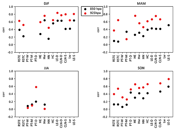 ), the correlation is higher than 0.4 under winter lows. The correlation between the wind speeds at the 1000 and 925 hPa levels is 0.6-0.8. Again, very low correlation is found under PT-W, PT-M and Hw during summer. Under the high group the correlation between the wind speeds at the 1000 and 925 hPa levels is ~ 0.6 during all seasons, except summer.
 |
Fig. (7) The correlation between wind speed at 1000,925 hPa levels (red) and 1000,850 hPa levels (black) at 0Z. The correlation was calculated when more than 30 events were found. The number of events is displayed in Table 2 and Table S1. |
4.3. The Three Categories of Cross Angles (CA) From Radiosonde Profiles
The study of CA and wind speed according to frequent synoptic classes and seasons at 12Z (LT = Z + 3h in summer and LT = Z + 2 h in winter) indicates three typical CA categories based on the relation between 1000 hPa and 850 hPa wind directions (hereafter, dd1000, dd850). These categories are characterized as follows:
a) “Low troposphere inversion” category: dd1000 is relatively constant in the West-Northwest directions while dd850 has a much wider range (0°-45°, 135°-360°).
The synoptic classes RSTE, PT-W, PT-M, PT-D and HW are mostly in this category.
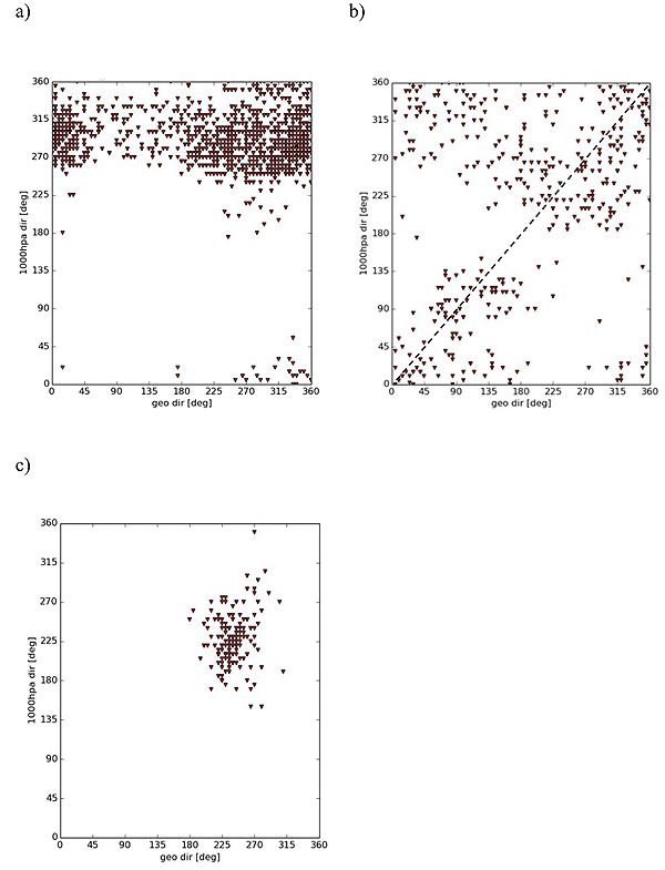
An example is given in Fig. (8a ) of a weak Persian Trough (PT-W) during JJA. As expected, during the summer in Israel the horizontal temperature gradient between sea and land creates strong sea breezes [15Skibin D, Hod A. Subjective analysis of mesoscale flow patterns in northern Israel. J Appl Meteorol 1979; 18: 329-38.
[http://dx.doi.org/10.1175/1520-0450(1979)018<0329:SAOMFP>2.0.CO;2] , 35Doron E, Neumann J. Land and mountain breezes with special attention to Israel Mediterranean Coastal plain. Isr Meteorol Res Papers 1977; 1: 109-22., 36Alpert P. The combined use of three different approaches to obtain the best estimate of meso-β surface winds above complex terrain. Boundary-Layer Meteorol 1988; 45(3): 291-305.
[http://dx.doi.org/10.1007/BF01066674] ], leading to dd1000 in the range of 240°-315° (Fig. 8a). No North-easterly to Easterly winds are found at 850 hPa (Fig. 8a), since the subtropical high dominates at the higher levels [32Dayan U, Rodnizky J. The temporal behavior of the atmospheric boundary layer in Israel. J App Met 1999; 38: 830.
[http://dx.doi.org/10.1175/1520-0450(1999)038<0830:TTBOTA>2.0.CO;2] ]. The lack of a strong correlation between wind at 1000 and 850 is related to a significant change of thermal stability from unstable to stable from 1000 hPa to 850 hPa. It was shown [16Dayan U, Shenhav R, Graber M. The spatial and temporal behavior of the mixed layer in Israel. J Appl Meteorol 1988; 27: 1382-94.
[http://dx.doi.org/10.1175/1520-0450(1988)027<1382:TSATBO>2.0.CO;2] , 31Arya SP. Introduction to Micrometeorology 1988; 307.] that the mixing layer height at BD is 760 ± 360 m under PT-W and 790 ± 310 m under PT-D: i.e. the inversion prevents efficient interaction between 1000 and 850 hPa winds, since the height of 850 hPa is ~1500 m. Inspection of CA925 results reveal relatively small values; 74-100% of the events show magnitudes lower than 60°. Under PT-W and PT-M very low correlation was found between the wind speeds at the 1000 and 925 hPa levels or between the 1000 and 850 hPa levels. Relatively low speed (~ 4 m/s) was found at most of the events under these classes during JJA according to scatter plots (not shown).
b) “Not well-defined” category: No steady unidirectional flow at 1000 hPa or at 850 hPa. In some of the events, dd1000 is nearly equal to dd850 (dashed line Fig. 8b). This category relates to the classes RSTc, RSTE, HE and HN.
The inversion height over Israel during the transitional seasons is at ~1300 ± 780m under weak RST and 920 ±730 m under Highs or weak pressure gradients [16Dayan U, Shenhav R, Graber M. The spatial and temporal behavior of the mixed layer in Israel. J Appl Meteorol 1988; 27: 1382-94.
[http://dx.doi.org/10.1175/1520-0450(1988)027<1382:TSATBO>2.0.CO;2] ]. According to this data, the inversion height may be above or below 850 hPa; therefore, no simple rule can be made for dd1000 according to season and synoptic class or dd850 at 12Z. This fact was found in a separate study of coastal surface winds [11Berkovic S. Synoptic classes as a predictor of hourly surface wind regimes: The case of the central and southern israeli coastal plains. J App Met Climatol 2016; 55(7): 1533 2016; 55(7): 1533. http://dx.doi.org/10.1175/JAMC-D-16-0093.1]. The increased height of the mixing layer may explain relatively high correlation (0.5-0.8) under the various highs (Figs. 6, 7) between wind speeds at the 1000 and 925hPa levels at 0, 12Z. At 12Z there is no defined surface wind direction under RST, HE and HN, when the synoptic wind and the local wind are often even in opposite directions (northerly or easterly synoptic wind versus westerly local wind). However, during the evening and night hours, when the synoptic wind and the local wind are parallel, the surface wind direction is mostly East to Southeast [11Berkovic S. Synoptic classes as a predictor of hourly surface wind regimes: The case of the central and southern israeli coastal plains. J App Met Climatol 2016; 55(7): 1533 2016; 55(7): 1533. http://dx.doi.org/10.1175/JAMC-D-16-0093.1]. Fig. (8b) demonstrates this category under HN during DJF. Similar behavior was found under HE and RSTC.
c) “Cyclone activity” category: dd1000 and dd850 are related due to strong vertical mixing during winter lows. Therefore dd1000 can be determined by dd850.
The tops of the mixing layer under winter lows are relatively high, i.e., 1320 ± 940 m at the warm sector of a cold low and 1580 ± 840 m behind the cold front [16Dayan U, Shenhav R, Graber M. The spatial and temporal behavior of the mixed layer in Israel. J Appl Meteorol 1988; 27: 1382-94.
[http://dx.doi.org/10.1175/1520-0450(1988)027<1382:TSATBO>2.0.CO;2] ].
In this case dd1000 and dd850 have similar wind directions within the range of 180-270°, according to the known cyclone flow next to the surface; south westerly winds when the low approaches the region and afterwards wind turning to westerly and north westerly wind when the low advances to the east of Israel [37Ziv B, Yair Y. An introduction to meteorology 1994. (in Hebrew)]. Fig. (8c) exemplifies this behavior under CLN-D during DJF. Relatively small CA925 and CA850 were found at most of the events at 12Z. At 0Z, due to the effect of the mesoscale winds during the night, larger CA values were obtained. The correlation between the wind speeds at the 1000 and 925 hPa levels, or between the 1000 and 850 hPa winds under winter lows is relatively high (0.6-0.8) at 12Z and 0Z (Figs. 6, 7).
4.4. Wind Verification of Era-interim .vs. Radiosonde Data
In order to evaluate the ERA-Interim horizontal wind data, a comparison of reanalysis vs. BD radiosonde measurements was performed. The comparison was made at each of the pressure levels 1000, 925, 850 hPa firstly according to seasons and hours and secondly according to seasons, synoptic classes and hours. This method enables the comparison of our results to other verifications of ERA-Interim at similar locations around the world according to the open literature. Validation of CA may suffer from error cancelation, and therefore the verification of the prediction at each level is preferable. Good prediction of wind direction at each level will be followed by good prediction of CA, since CA is a subtraction of the wind direction at two levels.
Table 8 shows the speed verification at 12Z (a) and 0Z (b) according to the statistical parameters: bias, RMSE, correlation, slope and intercept. At 12Z, no significant bias was obtained (bias < 0.5 m/s). The RMSE increases with height from 1.5 to 1.9 m/s for all seasons. The slope is less than 1 and increases with height, as the reanalysis under-estimates the wind speed especially at 1000hPa. The best result is obtained during DJF (a~ 0.8) and MAM (0.6 <a<0.8). During JJA at 1000 hPa the reanalysis shows constant wind speed ~ 4 m/s since it does not include the mesoscale effects. The correlation increases with height and the highest values are obtained during DJF and MAM (0.7-0.9). Underestimation of strong winds was found by Ruti et al. [38Ruti PM, Marullo S, D’Ortenzio F, Tremant M. Comparison of analyzed and measured wind speeds in the perspective of oceanic simulations over the Mediterranean basin: Analyses, QuikSCAT and buoy data. J Mar Syst 2008; 70: 33-48.
[http://dx.doi.org/10.1016/j.jmarsys.2007.02.026] ] while comparing buoys and QuickSCAT data to ECMWF analysis and ERA40 reanalysis results. On the average, the underestimation is about 30%. The following statistical parameters for the operational ECMWF and the ERA40 model surface winds (~ 1000 events) were reported: correlation coefficients 0.8-0.9, 0.6-0.8; RMSE 1.8-2.8, 2.9-3.9 m/s; slopes 0.61-0.85, 0.37-0.60 and intercepts of 0.66-2.38, 0.77-1.60, respectively.

a) 12Z wind speed verification. N is the number of events. The bias is calculated according to measurements – model results. Corr- correlation. a - slope b – intercept according to scatter plot of measurements (x axis) versus model results. b) same as a) at 0Z. c) same as a) for wind direction at 12Z. d) same as c) at 0Z. a) wind speed 12Z


At 0Z the bias increases to ~ 1 m/s at 850 hPa during JJA. The RMSE increases with height from 1 to 2 m/s. The correlation increases with height from 0.6 to 0.9 except during JJA (0.3-0.8). The wind speed is under-estimated by the reanalysis. The results improve with height according to the increasing slope values (0.5<a<0.8), except during JJA (0.2< a<0.6); these results are similar to those obtained at 12Z (Table 8a).
Tables 8c, d display wind direction verifications. Table 8c displays 12Z results. No significant bias was obtained. The RMSE is 60° – 30° and the correlation is 0.9-0.8. The slope is 0.8-1, and indicates good prediction at all levels, especially 925 and 850 hPa. BD is located in a flat coastal area where during daytime the synoptic wind and the local wind (sea breeze and upslope wind) both have a westerly component. Therefore, even coarse resolution reanalysis is able to predict well the nearly unidirectional local persistent flow next to the surface. Similar performance in reproducing the surface wind directions was also found at other sites over the Mediterranean by Ruti et al. [36Alpert P. The combined use of three different approaches to obtain the best estimate of meso-β surface winds above complex terrain. Boundary-Layer Meteorol 1988; 45(3): 291-305.
[http://dx.doi.org/10.1007/BF01066674] ]. 0Z results are displayed in Table 8d. The bias is negligible except under JJA at 1000 hPa, which indicates the inability of the reanalysis to include the land breeze and downslope winds along the shore. The RMSE is relatively low at 925 and 850 hPa (40°-20°); however it increases to 60°-90° during all seasons at 1000 hPa. This fact stresses the inability of the reanalysis to describe the local recirculation during the year. Accordingly high correlation (0.9-1.0) and slope (0.9-1.0) values are obtained at the higher levels (925, 850 hPa).
Ruti et al. [36Alpert P. The combined use of three different approaches to obtain the best estimate of meso-β surface winds above complex terrain. Boundary-Layer Meteorol 1988; 45(3): 291-305.
[http://dx.doi.org/10.1007/BF01066674] ] performed a comparison between QuickSCAT and ERA40 over a large domain of the Mediterranean Sea showing that the vector correlation tends to decrease from more than 0.85 in the offshore region to less than 0.5–0.6 near many coastal areas. This phenomenon was found for other regions in the world [39Perlin N, Samelson RM, Chelton DB. Scatterometer and model wind and wind stress in the Oregon–Northern California coastal zone. Mon Weather Rev 2004; 132: 2110-29.
[http://dx.doi.org/10.1175/1520-0493(2004)132<2110:SAMWAW>2.0.CO;2] ]. The coastal area, where the interaction between the atmospheric flow and the topography dominates, shows low correlation values which may arise from the coarseness of the model resolution relative to the horizontal scale (< 10 km) for local processes. This decrease is less evident in coastal regions dominated by the Mistral in the gulf of Lion or Etesian winds in the Levantine basin. Along the Israeli coast the vector correlation is 0.8-0.85.
Zecchetto and Accadia [40Zecchetto S, Accadia C. Diagnostics of T1279 ECMWF analysis winds in the Mediterranean basin by comparison with ASCAT 12.5 km winds. Q J R Meteorol Soc 2014; 140: 2506-14.
[http://dx.doi.org/10.1002/qj.2315] ] studied the model’s prediction as a function of distance from the coast. They compared 2 years of ECMWF T1279 (≈16 km grid size [41Ecmwf.int. What is the horizontal resolution of the data? | ECMWF. [online] 2017. Available at:
https:/ /www.ecmwf.int /en/what- horizontal-resolution -data]) global model data and satellite scatterometer (ASCAT) measurements. The ASCAT–ECMWF mean relative bias and centered root mean square deviation (RMSDc) of wind speed, normalized by scatterometer wind speed wsc, ws/wsc and RMSDc_ws/wsc, were 7 and 23%. The dependence of both ws/wsc and RMSDc_ws/wsc on the distance from the coast, indicates that the coastal areas is the main source of discrepancy between the two datasets. From 50 to 200 km away from coast, RMSDc_ws/wsc decreases from 40 to 25% and ws/wsc from 8 to 4%. The seasonal variation of RMSDc_ws/wsc shows higher values during the warm season (April to October). The authors suggest that the local coastal circulations like land/sea breezes could explain the mismatch between model and observations.
Since inference according to synoptic classes is considered, further investigation of the reanalysis prediction according to synoptic class, season and hour was performed. The RMSE of the wind speed at 12Z and 0Z are presented in Figs. (9a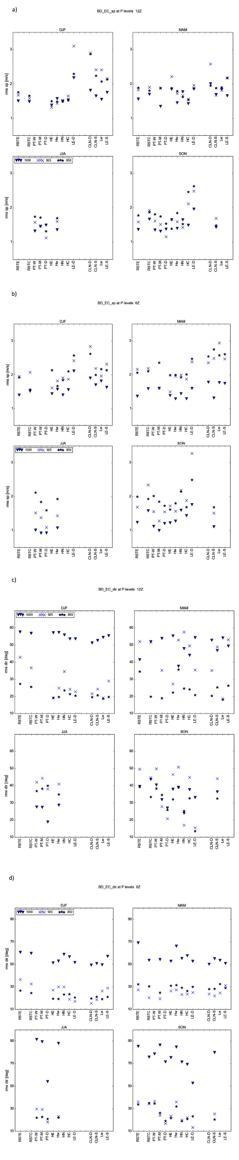 , b) respectively. The maximum RMSE (2 – 3 m/s) was obtained at 12Z under LE-D and CLN-D during DJF, SON. Deep winter lows are accompanied by high wind speeds (~ 10 m/s at surface level) and accordingly have the highest RMSE. The wind speed increases with height and the RMSE changes accordingly. The other synoptic classes have lower and similar RMSE at all levels (1.5-2 m/s); usually RMSE at 1000 hPa is the lowest during all seasons.

Similarly, at 0Z, CLN-D and LE-D show the highest RMSE (2-3 m/s) during all seasons except JJA. The RMSE under other synoptic classes is 1-2 m/s with the lowest RMSE at 1000 hPa.
The RMSE of the wind direction at 12Z and 0Z is shown in Figs. (7c, d). At 12Z, the best prediction of the wind direction is obtained at 1000 hPa during JJA under PT’s and Hw (20°-30°). As previously explained, this stems from the fact that the synoptic and the meso winds have similar directions. However, during DJF and MAM the RMSE at 1000 hPa is 50°-60° under all synoptic classes. The prediction at 1000 hPa under PT’s and Hw during JJA is better than that of deep winter lows during DJF in accordance with higher correlation due to the persistence of NW surface winds during JJA (0.88-0.91 for PT’s and Hw versus 0.71-0.78 for winter lows). At 925 hPa during MAM and SON the highest RMSE (50°) is obtained under synoptic classes with shallow pressure gradients (RSTE RSTC PT-W Hw Hc CLN-S LE-S). At 850 hPa good prediction (20°-30°) is obtained during DJF, MAM under all synoptic classes. The number of PT’s and Hw events is higher during SON relative to MAM and therefore SON RMSE values are similar to those at JJA. At 0Z the RMSE at 925 and 850 hPa is relatively low (40°-20°), however the RMSE at 1000 hPa is relatively high (60°-90°). The highest RMSE values during JJA, SON at 1000 hPa 0Z again exemplify the fact that the reanalysis does not include mesoscale effects.
The factors causing these deficiencies were mentioned in previous works. The model does not include subgrid scales smaller than ~ 80 km and the explicit topography is smoothed and not fully described [42Kara AB, Wallcraft AJ, Barron CN, Hurlburt HE, Bourassa MA. Accuracy of 10m winds from satellites and NWP products near land-sea boundaries. J Geophys Res 2008; 113: C10020.
[http://dx.doi.org/10.1029/2007JC004516] ]. It is well known that the actual effective resolution for any model is of the order of 5-10 times the grid spacing. Deficient theoretical description of the turbulent fluctuations next to the surface increases the prediction error of the surface wind direction [43Salameh T, Drobinski P, Vrac M, Naveau P. Statistical downscaling of near-surface wind over complex terrain in southern France. Meteorol Atmos Phys 2009; 103: 253-65.
[http://dx.doi.org/10.1007/s00703-008-0330-7] ]. The RMSE is affected by the hilly terrain and drag over land enhancing directionality [44Sun C, Monahan AH. Statistical downscaling prediction of sea surface winds over the global ocean. J Clim 2013; 26: 7938.
[http://dx.doi.org/10.1175/JCLI-D-12-00722.1] ], therefore a high resolution model is needed in order to better simulate these parameters.
5. SUMMARY
This work has considered two aspects pertaining to the feasibility of statistically downscaling surface wind according to synoptic class, season and hour from 925, 850 hPa wind with the stress on extreme wind events: 1. wind veering and wind speed correlation in the low stratosphere from radiosonde data 2. the ability of ERA-Interim analysis to predict low stratosphere wind. The CA925, CA850 and wind speed correlations were calculated from radiosonde data at Beit Dagan (BD) a station on the Israeli coastal plain. Afterwards, a comparison of ERA-Interim to radiosonde horizontal wind at 1000, 925 and 850 hPa levels was performed according to season, hour (0, 12Z) and synoptic class. The comparison was performed at each pressure level individually in order to facilitate comparison to open literature works and to avoid error cancellation. To the best of our knowledge no previous quantitative verification of wind profile qualities has been performed for this area.
Two extreme categories were found. Under the first category, “low troposphere inversion”, strong thermal inversion prevents efficient interaction between these two levels and the CA values are as high as ±180º. 75-100% of the CA925 under PT’s and Hw magnitudes were smaller than 60°; however, only 49-70% CA850 magnitudes under Hw were smaller than 60°. Very low correlation between wind speeds at 1000 and 925 hPa levels was found under PT-W, PT-M and Hw during summer, the wind speed at each of these levels is relatively weak 4± 2 m/s at most of the events (according to scatter plots of wind speed, not shown). In the second “cyclone activity” category, as expected, strong vertical mixing creates higher resemblance between the winds along the vertical profile. In this category, 65-93% of the CA925 and CA850 magnitudes are smaller than 60º. Under extreme wind events of winter lows at 925 and 850 hPa at 12Z 72-100% of the CA925 or CA850 magnitudes are smaller than 60º. High correlation is found between the wind speeds at the two sets of levels (0.6-0.8).
At 0Z, due to increased thermal stability next to the surface, larger values of CA850 and CA925 were obtained under all synoptic classes, and only 49-82% of CA925 and 35-68% of CA850 magnitudes were smaller than 60°. Extreme wind events under winter lows at 0Z still show relatively high CA values, 60-88% of CA925 and only 42-74% of CA850 magnitudes are lower than 60°. Therefore direct inference of wind direction from 925, 850 hPa data at 0Z under winter lows is questionable. On the other hand, wind speed inference may still be possible, due to high correlation between wind speeds at the two sets of levels during the night.
To summarize, an inspection of the wind speed correlation and CA at 12Z reveals that under winter lows the wind speed correlation is high and the turning of the wind is in general small, which may allow derivation of wind close to the ground from the higher levels. At 0Z, high correlation of wind speed at the two sets of levels was found under winter lows, i.e. wind speed inference may be possible. At 12Z relatively small CA925 and very low wind speed correlation were found under high to the west and PTs, i.e. wind direction inference may be possible.
A thorough study of the ERA-Interim prediction of wind speed and direction at 1000, 925, 850 hPa according to season and hour has shown good prediction of the wind direction at 925 and 850 hPa (RMSE 20°-60°) at 12Z and (RMSE 20°-40°) at 0Z. At 1000 hPa at 12Z good prediction is obtained for all synoptic classes (20°- 60°), especially under PT’s and Hw during JJA (20°-30°). However, at 0Z, the quality of the prediction is lower (RMSE 60°-90°) for all seasons and synoptic classes. Referring to the wind speed prediction, the RMSE is 1-2 m/s for all seasons and synoptic classes except winter lows with 2-3 m/s RMSE at 0, 12Z at all levels. According to scatter plots, the reanalysis under-predicts the wind speed for all seasons. The slope is 0.5-0.8 at all seasons and levels except JJA. During JJA at 1000 hPa the mesoscale effects were not detected by the analysis and constant wind speed ~ 4 m/s is obtained. i.e., for 1000 hPa during JJA at 12Z better prediction of wind direction and poorer prediction of wind speed is obtained.
CONCLUSION
According to the CA calculations, wind speed correlation and the analysis verification, inference of surface wind at 12Z from 925 or 825 hPa winds may be possible under winter lows. Wind direction inference may be possible at 12Z from 925 hPa winds under high to the west and Persian troughs. Wind speed inference may be possible under lows at 0Z. As a result of the under estimation of the wind speed at the higher levels (925, 850 hPa), wind speed should be inferred by interpolation, according to historical data from measurements or high resolution model. Under other synoptic classes, surface winds may be estimated according to statistics of measurements (Berkovic 2016). Around 50% of the 3 hourly events under the frequent synoptic classes can be characterized by their average wind surface data with relatively small standard deviation (std) of wind direction (std < 60º) and speed (std ~ 1-2 m/s).
Other objective statistical downscaling methods and other predictors such as mixing height, wind, temperature and humidity should be considered. A few examples of objective statistical algorithms [45Trzaska S, Schnarr E. A review of downscaling methods for climate change projections. CIESIN report 2014. http:// www.ciesin.org /documents/ Downscaling_ CLEARED_000.pdf, 46Vandal T, Bhatia U, Ganguly AR. Statistical downscaling in climate with state-of-the-art scalable machine learning Ch.4. in Large-Scale Machine Learning in the Earth Sciences
Edited by Ashok N. Srivastava, Ramakrishna Nemani and Karsten Steinhaeuser 2017.] are SOM [14Berkovic S. Winter wind regimes over Israel using self-organizing maps. J Appl Meteorol Climatol 2017; 56: 2671-91.
[http://dx.doi.org/10.1175/JAMC-D-16-0381.1] , 47Horton DE, Johnson NC, Singh D, Swain DL, Rajaratnam B, Diffenbaugh NS. Contribution of changes in atmospheric circulation patterns to extreme temperature trends. Nature 2015; 522(7557): 465-9.
[http://dx.doi.org/10.1038/nature14550] [PMID: 26108856] , 48Yin C. Application of SOM to statistical downscaling of major regional climate variables 2011.
Available from: http:// researchcommons. waikato.ac.nz/ handle/ 10289/ 5733], Bayesian inference methods [43Salameh T, Drobinski P, Vrac M, Naveau P. Statistical downscaling of near-surface wind over complex terrain in southern France. Meteorol Atmos Phys 2009; 103: 253-65.
[http://dx.doi.org/10.1007/s00703-008-0330-7] , 49Manor A, Berkovic S. Bayesian Inference aided analog downscaling for near-surface winds in complex terrain. Atmos Res 2014; 164-165: 27-36.
[http://dx.doi.org/10.1016/j.atmosres.2015.04.014] ], non-parametric regression based on generalized additive models [40Zecchetto S, Accadia C. Diagnostics of T1279 ECMWF analysis winds in the Mediterranean basin by comparison with ASCAT 12.5 km winds. Q J R Meteorol Soc 2014; 140: 2506-14.
[http://dx.doi.org/10.1002/qj.2315] ] and Cumulative Distribution Function transform [7Lavaysse C, Vrac M, Drobinski P, Lengaigne M, Vischel T. Statistical downscaling of the french mediterranean climate: Assessment for present and projection in an anthropogenic scenario. Nat Hazards Earth Syst Sci 2012; 12: 651-70.
[http://dx.doi.org/10.5194/nhess-12-651-2012] ]. Dynamical downscaling may provide better prediction of mesoscale effects and will enable direct prediction of surface winds at the expense of much heavier computational effort at higher horizontal resolution (1-3 km). High resolution models in climate projections have started to be employed in recent years [50Mizielinski MS, Roberts MJ, Vidale PL, et al. High-resolution global climate modelling: The UPSCALE project, a large-simulation campaign. Geosci Model Dev 2014; 7: 1629-40.
[http://dx.doi.org/10.5194/gmd-7-1629-2014] -52Flaounas E, Drobinski P, Bastin S. Dynamical downscaling of IPSL-CM5 CMIP5 historical simulations over the Mediterranean: Benefits on the representation of regional surface winds and cyclogenesis. Clim Dyn 2012.
[http://dx.doi.org/10.1007/s00382-012-1606-7] ]. According to Li et al. [53Li H, Kanamitsu M, Hong SY, Yoshimura K, Cayan CR, Misra V. A high-resolution ocean-atmosphere coupled downscaling of the present climate over California. Clim Dyn 2014; 42: 701-14.
[http://dx.doi.org/10.1007/s00382-013-1670-7] ] high resolution and ocean-atmosphere coupled models are necessary to predict future climate in coastal areas.
CONSENT FOR PUBLICATION
Not applicable.
CONFLICT OF INTEREST
The authors declare that there is no conflict of interest, financial or otherwise.
SUPPLEMENTARY MATERIAL
Supplementary material is available on the publishers Web site along with the published article.
ACKNOWLEDGEMENTS
The authors thank H. Saaroni, B. Ziv, I. Osetinsky and T. Harpaz for providing the synoptic classification data. The authors also thank the Israeli Ministry of Science and Technology for funding through MOST grant 605404541.
REFERENCES
| [1] | Navarra A, Tubiana L. Regional Assessment of Climate Change in the Mediterranean 2013. |
| [2] | Lionello P. The clime of the Mediterranean Region 2012. |
| [3] | Kit K. Marine Policy Plan for Israel 2014.http:// msp-israel.net.technion.ac.il /files/2014 /12/ATOS-report -final.pdf |
| [4] | Somot S, Sevault F, Deque M, Crepon M. 21st century climate change scenario for the Mediterranean using a coupled atmosphere-ocean regional climate model. Global Planet Change 2008; 63: 112-26. [http://dx.doi.org/10.1016/j.gloplacha.2007.10.003] |
| [5] | Herrmann M, Somot S, Calmanti S, Dubois C, Sevault F. Representation of spatial and temporal variability of daily wind speed and of intense wind events over the Mediterranean Sea using dynamical downscaling: Impact of the regional climate model configuration. Nat Hazards Earth Syst Sci 2011; 11: 1983-2001. [http://dx.doi.org/10.5194/nhess-11-1983-2011] |
| [6] | Najac J, Lacb C, Terraya L. Impact of climate change on surface winds in France using a statistical-dynamical downscaling method with mesoscale modeling. Int J Climatol 2011; 31: 415-30. [http://dx.doi.org/10.1002/joc.2075] |
| [7] | Lavaysse C, Vrac M, Drobinski P, Lengaigne M, Vischel T. Statistical downscaling of the french mediterranean climate: Assessment for present and projection in an anthropogenic scenario. Nat Hazards Earth Syst Sci 2012; 12: 651-70. [http://dx.doi.org/10.5194/nhess-12-651-2012] |
| [8] | Hochman A, Harpaz T, Saaroni H, Alpert P. Synoptic classification in 21st Century CMIP5 predictions over the Eastern Mediterranean with focus on cyclones, accepted for publication Int. J Clim 2017. |
| [9] | Alpert P, Osetinsky I, Ziv B, Shafir H. Semi-objective classification for daily synoptic systems: Application to the Eastern Mediterranean climate change. Intern J Climatol 2004; 24: 1001-11.http:// www.tau.ac.il/ ~pinhas/papers/2004 /Alpert_et_al _IJC_2004a.pdf |
| [10] | Osetinsky I. Climate changes over the E. Mediterranean-A synoptic systems classification approach. Ph.D. thesis, Tel Aviv University, 2006: 153 pp. |
| [11] | Berkovic S. Synoptic classes as a predictor of hourly surface wind regimes: The case of the central and southern israeli coastal plains. J App Met Climatol 2016; 55(7): 1533 2016; 55(7): 1533. http://dx.doi.org/10.1175/JAMC-D-16-0093.1 |
| [12] | Zorita E, von Storch H. The analog method as a simple down-scaling technique: Comparison with more complicated methods. J Clim 1999; 12: 2474-89. [http://dx.doi.org/10.1175/1520-0442(1999)012<2474:TAMAAS>2.0.CO;2] |
| [13] | Huth R. Disaggregating climatic trends by classification of circulation patterns. Int J Climatol 2001; 21: 135-53. [http://dx.doi.org/10.1002/joc.605] |
| [14] | Berkovic S. Winter wind regimes over Israel using self-organizing maps. J Appl Meteorol Climatol 2017; 56: 2671-91. [http://dx.doi.org/10.1175/JAMC-D-16-0381.1] |
| [15] | Skibin D, Hod A. Subjective analysis of mesoscale flow patterns in northern Israel. J Appl Meteorol 1979; 18: 329-38. [http://dx.doi.org/10.1175/1520-0450(1979)018<0329:SAOMFP>2.0.CO;2] |
| [16] | Dayan U, Shenhav R, Graber M. The spatial and temporal behavior of the mixed layer in Israel. J Appl Meteorol 1988; 27: 1382-94. [http://dx.doi.org/10.1175/1520-0450(1988)027<1382:TSATBO>2.0.CO;2] |
| [17] | Zaiter DS, Al-Jumaily KJ. Characteristics of thermal wind over iraq. Inter J Sci Res Publ 2016; 6: 163-7. |
| [18] | weather.uwyo.edu weather.uwyo.edu http ://weather.uwyo.edu/ upperair/ |
| [19] | Holton JR. An Introduction to Dynamic Meteorology 4th ed. 2004. |
| [20] | Savijarvi H. Model predictions of coastal winds in a small scale. Tellus, Ser A, Dyn Meterol Oceanogr 2004; 56(4): 287-95. [http://dx.doi.org/10.1111/j.1600-0870.2004.00069.x] |
| [21] | Truitt J. Using the thermal wind relationship to improve offshore and coastal forcasts of extratropical cyclone surface winds. Nat Wea Dig 2008; 32(2): 153-65. |
| [22] | Ramella Pralungo L, Haimberger L. New estimates of tropical mean temperature trend profiles from zonal mean historical radiosonde and pilot balloon wind shear observations. J Geophys Res Atmos 2015; 120: 3700-13. [http://dx.doi.org/10.1002/2014JD022664] |
| [23] | Wang S, O’Neill LW, Jiang Q, et al. A regional real time forecast of marine boundary layers during VOCALS-Rex. Atmos Chem Phys 2011; 11: 421-37. [http://dx.doi.org/10.5194/acp-11-421-2011] |
| [24] | Scipy.org https:// docs.scipy.org /doc/scipy -0.14.0/reference /generated/ scipy.stats.pearsonr.html |
| [25] | Apps.ecmwf.int. ERA Interim, Daily. [online] 2017. Available at: http:// apps.ecmwf.int/ datasets/data /interim-full- daily/ |
| [26] | Berrisford P, Dee DP, Poli P, et al. The ERA-interim archive version 2.0 2011. Available from: http:// www.ecmwf.int/ en/elibrary/ 8174-era-interim -archive-version-20 |
| [27] | Zhemin T, Juan F, Rongsheng W. Nonlinear Ekman layer theories and their applications. Acta Meteorol Sin 2006; 20: 209-22. |
| [28] | Stull RB. Introduction to boundary layer meteorology 2003. |
| [29] | Beljaars A. The parametrization of the planetary boundary layer 1992. Available from: https:// www.ecmwf.int /sites/ default/ files/elibrary/ 2002/16959-parametrization -planetary- boundary- layer.pdf |
| [30] | Plant B. Boundary Layer Parameterization 2014. Available from: http:// www.met.reading .ac.uk/~ sws00rsp/teaching /nanjing/blayer.pdf |
| [31] | Arya SP. Introduction to Micrometeorology 1988; 307. |
| [32] | Dayan U, Rodnizky J. The temporal behavior of the atmospheric boundary layer in Israel. J App Met 1999; 38: 830. [http://dx.doi.org/10.1175/1520-0450(1999)038<0830:TTBOTA>2.0.CO;2] |
| [33] | Uzan L, Egert S, Alpert P. Ceilometer evaluation of the East Mediterranean summer boundary layer height – first study of two Israeli sites. Atmos Meas Tech Discuss 2016; 9: 4387-98. [http://dx.doi.org/10.5194/amt-9-4387-2016] |
| [34] | Ziv B, Saaroni H, Alpert P. The factors governing the summer regime of the eastern Mediterranean. Int J Climatol 2004; 24: 1859-71. [http://dx.doi.org/10.1002/joc.1113] |
| [35] | Doron E, Neumann J. Land and mountain breezes with special attention to Israel Mediterranean Coastal plain. Isr Meteorol Res Papers 1977; 1: 109-22. |
| [36] | Alpert P. The combined use of three different approaches to obtain the best estimate of meso-β surface winds above complex terrain. Boundary-Layer Meteorol 1988; 45(3): 291-305. [http://dx.doi.org/10.1007/BF01066674] |
| [37] | Ziv B, Yair Y. An introduction to meteorology 1994. (in Hebrew) |
| [38] | Ruti PM, Marullo S, D’Ortenzio F, Tremant M. Comparison of analyzed and measured wind speeds in the perspective of oceanic simulations over the Mediterranean basin: Analyses, QuikSCAT and buoy data. J Mar Syst 2008; 70: 33-48. [http://dx.doi.org/10.1016/j.jmarsys.2007.02.026] |
| [39] | Perlin N, Samelson RM, Chelton DB. Scatterometer and model wind and wind stress in the Oregon–Northern California coastal zone. Mon Weather Rev 2004; 132: 2110-29. [http://dx.doi.org/10.1175/1520-0493(2004)132<2110:SAMWAW>2.0.CO;2] |
| [40] | Zecchetto S, Accadia C. Diagnostics of T1279 ECMWF analysis winds in the Mediterranean basin by comparison with ASCAT 12.5 km winds. Q J R Meteorol Soc 2014; 140: 2506-14. [http://dx.doi.org/10.1002/qj.2315] |
| [41] | Ecmwf.int. What is the horizontal resolution of the data? | ECMWF. [online] 2017. Available at: https:/ /www.ecmwf.int /en/what- horizontal-resolution -data |
| [42] | Kara AB, Wallcraft AJ, Barron CN, Hurlburt HE, Bourassa MA. Accuracy of 10m winds from satellites and NWP products near land-sea boundaries. J Geophys Res 2008; 113: C10020. [http://dx.doi.org/10.1029/2007JC004516] |
| [43] | Salameh T, Drobinski P, Vrac M, Naveau P. Statistical downscaling of near-surface wind over complex terrain in southern France. Meteorol Atmos Phys 2009; 103: 253-65. [http://dx.doi.org/10.1007/s00703-008-0330-7] |
| [44] | Sun C, Monahan AH. Statistical downscaling prediction of sea surface winds over the global ocean. J Clim 2013; 26: 7938. [http://dx.doi.org/10.1175/JCLI-D-12-00722.1] |
| [45] | Trzaska S, Schnarr E. A review of downscaling methods for climate change projections. CIESIN report 2014. http:// www.ciesin.org /documents/ Downscaling_ CLEARED_000.pdf |
| [46] | Vandal T, Bhatia U, Ganguly AR. Statistical downscaling in climate with state-of-the-art scalable machine learning Ch.4. in Large-Scale Machine Learning in the Earth Sciences Edited by Ashok N. Srivastava, Ramakrishna Nemani and Karsten Steinhaeuser 2017. |
| [47] | Horton DE, Johnson NC, Singh D, Swain DL, Rajaratnam B, Diffenbaugh NS. Contribution of changes in atmospheric circulation patterns to extreme temperature trends. Nature 2015; 522(7557): 465-9. [http://dx.doi.org/10.1038/nature14550] [PMID: 26108856] |
| [48] | Yin C. Application of SOM to statistical downscaling of major regional climate variables 2011. Available from: http:// researchcommons. waikato.ac.nz/ handle/ 10289/ 5733 |
| [49] | Manor A, Berkovic S. Bayesian Inference aided analog downscaling for near-surface winds in complex terrain. Atmos Res 2014; 164-165: 27-36. [http://dx.doi.org/10.1016/j.atmosres.2015.04.014] |
| [50] | Mizielinski MS, Roberts MJ, Vidale PL, et al. High-resolution global climate modelling: The UPSCALE project, a large-simulation campaign. Geosci Model Dev 2014; 7: 1629-40. [http://dx.doi.org/10.5194/gmd-7-1629-2014] |
| [51] | Lader R, Walsh JE, Bhatt US, Bieniek PA. Projections of twenty-first-century climate extremes for alaska via dynamical downscaling and quantile mapping. JAMC 2017; 56: 2393. |
| [52] | Flaounas E, Drobinski P, Bastin S. Dynamical downscaling of IPSL-CM5 CMIP5 historical simulations over the Mediterranean: Benefits on the representation of regional surface winds and cyclogenesis. Clim Dyn 2012. [http://dx.doi.org/10.1007/s00382-012-1606-7] |
| [53] | Li H, Kanamitsu M, Hong SY, Yoshimura K, Cayan CR, Misra V. A high-resolution ocean-atmosphere coupled downscaling of the present climate over California. Clim Dyn 2014; 42: 701-14. [http://dx.doi.org/10.1007/s00382-013-1670-7] |