- Home
- About Journals
-
Information for Authors/ReviewersEditorial Policies
Publication Fee
Publication Cycle - Process Flowchart
Online Manuscript Submission and Tracking System
Publishing Ethics and Rectitude
Authorship
Author Benefits
Reviewer Guidelines
Guest Editor Guidelines
Peer Review Workflow
Quick Track Option
Copyediting Services
Bentham Open Membership
Bentham Open Advisory Board
Archiving Policies
Fabricating and Stating False Information
Post Publication Discussions and Corrections
Editorial Management
Advertise With Us
Funding Agencies
Rate List
Kudos
General FAQs
Special Fee Waivers and Discounts
- Contact
- Help
- About Us
- Search


The Ergonomics Open Journal
(Discontinued)
ISSN: 1875-9343 ― Volume 11, 2018
Forecasting Hourly Patient Visits in the Emergency Department to Counteract Crowding
Morten Hertzum*
Abstract
Background:
Emergency Department (ED) crowding is a frequent problem that causes prolonged waiting and increased risk of adverse events. While the number of daily and monthly patient arrivals can be forecasted with good accuracy, ED clinicians need hourly forecasts in their ongoing scheduling and rescheduling of their work.
Objective:
We aim to assess whether the hour-by-hour evolution in patient arrivals and ED occupancy can be accurately forecasted using calendar variables.
Method:
We obtained data about the patient visits at four Danish EDs from January 2012 to January 2015, a total of 393717 ED visits. The data for 2012-2014 were used to create linear regression models, autoregressive integrated moving average (ARIMA) models, and – for purposes of comparison – naïve models of hourly patient arrivals and ED occupancy. Using the models, patient arrivals and ED occupancy were forecasted for every hour of January 2015.
Results:
Hourly patient arrivals were forecasted with a mean percentage error of 47-58% (regression), 49-58% (ARIMA), and 60-76% (naïve). Increasing the forecasting interval decreased the mean percentage error. ED occupancy was forecasted with better accuracy by ARIMA than regression models. With ARIMA the mean percentage error of the forecasts of the hourly ED occupancy was 69-73% for three of the EDs and 101% for the last ED. Factors beyond calendar variables might possibly have improved the models of ED occupancy, provided that information about these factors had been consistently available.
Conclusion:
Hourly patient arrivals can be forecasted with decent accuracy. Forecasts of hourly ED occupancy are less accurate and their accuracy varies more across EDs.
Article Information

Identifiers and Pagination:
Year: 2017Volume: 10
First Page: 1
Last Page: 13
Publisher Id: TOERGJ-10-1
DOI: 10.2174/1875934301710010001
Article History:
Received Date: 27/09/2016Revision Received Date: 23/02/2017
Acceptance Date: 03/03/2017
Electronic publication date: 31/03/2017
Collection year: 2017
open-access license: This is an open access article distributed under the terms of the Creative Commons Attribution 4.0 International Public License (CC-BY 4.0), a copy of which is available at: https://creativecommons.org/licenses/by/4.0/legalcode. This license permits unrestricted use, distribution, and reproduction in any medium, provided the original author and source are credited.
* Address correspondence to this author at the Royal School of Library and Information Science, University of Copenhagen, Njalsgade 76, Bldg 4, Copenhagen, Denmark; Tel: 45 3234 1344; E-mail: hertzum@hum.ku.dk
| Open Peer Review Details | |||
|---|---|---|---|
| Manuscript submitted on 27-09-2016 |
Original Manuscript | Forecasting Hourly Patient Visits in the Emergency Department to Counteract Crowding | |
1. INTRODUCTION
The common entry point to hospitals for nearly all patients with acute problems is the emergency department (ED), which is a busy – sometimes hectic – place where severely injured persons may arrive at little notice, yet the bulk of the patients have unalarming injuries. EDs become crowded “when the identified need for emergency services exceeds available resources for patient care in the emergency department (ED), hospital, or both” [1American College of Emergency Physicians. Crowding. Ann Emerg Med 2006; 47(6): 585.
[http://dx.doi.org/10.1016/j.annemergmed.2006.02.025] [PMID: 16713796] , p. 585]. To counteract crowding, ED clinicians need advance warning of changes in the number of patient arrivals, the treatment capacity of the ED, and the possibility of transferring patients out of the ED. While the arrival of patients is determined by factors beyond the ED clinicians’ control, previous research has found consistent hour-of-the-day and day-of-the-week patterns in patient arrivals [2Hertzum M. Patterns in emergency-department arrivals and length of stay: Input for visualizations of crowding. Ergon Open J 2016; 9: 1-14.
[http://dx.doi.org/10.2174/1875934301609010001] -6Tandberg D, Qualls C. Time series forecasts of emergency department patient volume, length of stay, and acuity. Ann Emerg Med 1994; 23(2): 299-306.
[http://dx.doi.org/10.1016/S0196-0644(94)70044-3] [PMID: 8304612] ]. Such patterns enable forecasting. However, existing models for forecasting patient arrivals focus on forecasting daily [7Batal H, Tench J, McMillan S, Adams J, Mehler PS. Predicting patient visits to an urgent care clinic using calendar variables. Acad Emerg Med 2001; 8(1): 48-53.
[http://dx.doi.org/10.1111/j.1553-2712.2001.tb00550.x] [PMID: 11136148] -11Wargon M, Casalino E, Guidet B. From model to forecasting: a multicenter study in emergency departments. Acad Emerg Med 2010; 17(9): 970-8.
[http://dx.doi.org/10.1111/j.1553-2712.2010.00847.x] [PMID: 20836778] ] or monthly [5Rotstein Z, Wilf-Miron R, Lavi B, Shahar A, Gabbay U, Noy S. The dynamics of patient visits to a public hospital ED: a statistical model. Am J Emerg Med 1997; 15(6): 596-9.
[http://dx.doi.org/10.1016/S0735-6757(97)90166-2] [PMID: 9337370] , 12Bergs J, Heerinckx P, Verelst S. Knowing what to expect, forecasting monthly emergency department visits: A time-series analysis. Int Emerg Nurs 2014; 22(2): 112-5.
[http://dx.doi.org/10.1016/j.ienj.2013.08.001] [PMID: 24055373] ] arrivals. We focus on forecasting the hour-by-hour evolution in patient arrivals and ED occupancy to support ED clinicians in their ongoing scheduling and rescheduling of their work so that they can provide quality care and avoid crowding.
ED clinicians already use artifacts, such as whiteboards [13Hertzum M, Simonsen J. Visual overview, oral detail: The use of an emergency-department whiteboard. Int J Hum Comput Stud 2015; 82: 21-30.
[http://dx.doi.org/10.1016/j.ijhcs.2015.04.004] ], and procedures, such as triage [14Iserson KV, Moskop JC. Triage in medicine, part I: Concept, history, and types. Ann Emerg Med 2007; 49(3): 275-81.
[http://dx.doi.org/10.1016/j.annemergmed.2006.05.019] [PMID: 17141139] ], to schedule their work but whiteboards and triage help manage known patients. The aim of this study is to extend clinicians’ planning horizon a couple of hours into the future by providing forecasts of the arrival of patients who are yet unknown to the clinicians. Hourly forecasts are challenging because the noise caused by random variation may overshadow any pattern in the data. In this respect, forecasts of daily or monthly arrivals are likely easier but target decisions about staff allocation and the like, not the ongoing scheduling and rescheduling of how the available resources are divided among the patients in need of emergency services.
In this paper, we create models for forecasting the hour-by-hour evolution in patient arrivals, that is the number of people arriving in the ED for treatment, and ED occupancy, that is the accumulated increase since midnight in the number of patients in the ED. Of the several approaches to modeling ED operations we choose linear regression and time-series analysis, both recommended by Wiler et al. [15Wiler JL, Griffey RT, Olsen T. Review of modeling approaches for emergency department patient flow and crowding research. Acad Emerg Med 2011; 18(12): 1371-9.
[http://dx.doi.org/10.1111/j.1553-2712.2011.01135.x] [PMID: 22168201] ]. Accurate forecasts of hourly patient arrivals and ED occupancy will support clinicians in counteracting crowding. We assess the accuracy of the forecasts and discuss the possibilities of making them more accurate.
2. METHOD
The study was based on log data from visits at the four EDs in Region Zealand, one of five healthcare regions in Denmark. Prior to conducting the study we obtained approval from the healthcare region.
2.1. The ED Data
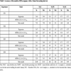
The four EDs were part of medium-sized hospitals and collectively served a population of approximately 817,000 citizens. To characterize the population served by each ED we obtained data from Statistics Denmark about the municipalities of Region Zealand and recalculated them into sums for the catchment areas of the EDs, see Table 1. ED1 served an older population with a higher frequency of chronic diseases and a lower employment rate. The three other EDs served rather similar populations. It may also be noted that in Denmark hospital care is financed via taxes. Thus, neither ED treatment nor treatment in an inpatient department is dependent on the patient’s personal wealth or insurance.
The EDs introduced the same electronic whiteboard in December 2009 (ED1), January 2010 (ED2), January 2011 (ED3), and May 2011 (ED4). The whiteboard supplemented the electronic patient record by providing procedural information about the patients, such as time of arrival, triage level, responsible physician, responsible nurse, current treatment activity, and time of departure. Whenever the content of the whiteboard changed, the change was automatically logged.
For the purpose of this study the whiteboard vendor produced a version of the logs from which all patient names, clinician names, and other information that might identify persons had been removed. These anonymized log data covered the period from January 2012 to January 2015. However, the data for January 2013 - January 2014 (ED1) and November 2013 - January 2014 (ED2-4) turned out to be incomplete and were discarded from the analysis. Thus, the analysis was based on 2.0 years of data from ED1 and 2.8 years of data from ED2, ED3, and ED4.
Each of the 10.15 million entries in the logs documented an event that changed the whiteboard content. A log entry consisted of a timestamp, the event type, any values associated with the event, and a system-generated identifier of the visit to which the event pertained. For example, the event type ‘LocationChanged’ along with the event value ‘Transferred’ indicated that the patient had been discharged from the ED. After removing 769 outliers (defined as visits longer than seven days, i.e. 53 times the median length of stay), the dataset comprised 393717 ED visits.
2.2. Models
We modeled the number of patient arrivals and the ED occupancy using calendar variables. We made all our models sensitive to the hour of the day and the day of the week because previous studies have found that ED arrivals vary significantly across these two calendar variables [2Hertzum M. Patterns in emergency-department arrivals and length of stay: Input for visualizations of crowding. Ergon Open J 2016; 9: 1-14.
[http://dx.doi.org/10.2174/1875934301609010001] -7Batal H, Tench J, McMillan S, Adams J, Mehler PS. Predicting patient visits to an urgent care clinic using calendar variables. Acad Emerg Med 2001; 8(1): 48-53.
[http://dx.doi.org/10.1111/j.1553-2712.2001.tb00550.x] [PMID: 11136148] ]. In addition, we included the month of the year in one of our models because several studies have found that ED arrivals also vary with this calendar variable [7Batal H, Tench J, McMillan S, Adams J, Mehler PS. Predicting patient visits to an urgent care clinic using calendar variables. Acad Emerg Med 2001; 8(1): 48-53.
[http://dx.doi.org/10.1111/j.1553-2712.2001.tb00550.x] [PMID: 11136148] , 8Jones SS, Thomas A, Evans RS, Welch SJ, Haug PJ, Snow GL. Forecasting daily patient volumes in the emergency department. Acad Emerg Med 2008; 15(2): 159-70.
[http://dx.doi.org/10.1111/j.1553-2712.2007.00032.x] [PMID: 18275446] , 11Wargon M, Casalino E, Guidet B. From model to forecasting: a multicenter study in emergency departments. Acad Emerg Med 2010; 17(9): 970-8.
[http://dx.doi.org/10.1111/j.1553-2712.2010.00847.x] [PMID: 20836778] , 12Bergs J, Heerinckx P, Verelst S. Knowing what to expect, forecasting monthly emergency department visits: A time-series analysis. Int Emerg Nurs 2014; 22(2): 112-5.
[http://dx.doi.org/10.1016/j.ienj.2013.08.001] [PMID: 24055373] ]. Our main interest was to forecast hourly arrivals and hourly occupancy but to assess the effect of the length of the forecasting interval on the accuracy of the models we made models for intervals of 1, 2, 4, 8, and 24 hours. For each forecasting interval, we made three models:
Linear regression, which fits a data series by a linear function of a set of predictors. As predictors we used indicator variables for the months of the year, the days of the week, and the hours of the day (in the analysis with a 2-hour forecasting interval the hours of the day were replaced with the 2-hour blocks of the day, and so forth for the 4-hour, 8-hour, and 24-hour forecasting intervals). We initially included all predictors and then applied the standard procedure of backward elimination [16Thompson ML. Selection of variables in multiple regression: Part I. A review and evaluation. Int Stat Rev 1978; 46(1): 1-19.
[http://dx.doi.org/10.2307/1402505] ] to sequentially remove the predictor that contributed the least to explaining the variance in the number of ED arrivals. This removal process continued as long as the significance of the F-test of the removed predictor exceeded 0.05. The resulting regression models included the predictors that contributed appreciably to explaining the variation in the number of ED arrivals. Regression models of the ED occupancy were created in a similar manner.
Autoregressive integrated moving average (ARIMA), which fits the data series with a seasonal and a non-seasonal component [17Box GE, Jenkins GM, Reinsel GC. Time series analysis: Forecasting and control. 4th ed. New York: Wiley 2008.
[http://dx.doi.org/10.1002/9781118619193] ]. The structure of an ARIMA model is represented as (p, d, q)×(P, D, Q)s where p, d, and q are the parameters of the non-seasonal component and give the order of autocorrelation, differencing, and moving averaging, respectively. P, D, and Q are the same parameters for the seasonal component, which has the periodicity s. The periodicity of the season must be specified, the other parameters were estimated with SPSS (version 22.0.0.0). To capture the daily as well as the weekly pattern in ED arrivals, we specified a season of a week consisting of 168 hours (in the analyses with forecasting intervals longer than 1 hour the season was specified as 84 / 2-hour, 42 / 4-hour, 21 / 8-hour, or 7 / 24-hour blocks). ARIMA models are a flexible and widely used means of modeling time series.
Naïve model, which for seasonal data series (e.g., those studied in this paper) uses as its forecast the observed value a season ago [18Makridakis S, Wheelright S, Hyndman RJ. Forecasting: Methods and applications. 3rd ed. New York: Wiley 1998.]. We used a season of one week and, thus, our naïve model forecasted that the number of ED arrivals at a specified time and day of week would equal the number of arrivals at the same time the previous week. The naïve model is a simple model against which to benchmark more sophisticated models.
2.3. Measures of Model Accuracy
We divided the data series for the four EDs into an estimation set, which consisted of the data from January 1, 2012, to December 31, 2014, and a forecasting set, which consisted of the data from January 1 to 31, 2015. The estimation set was used to estimate the model parameters and to measure how well the models fitted the data based on which they were made (the in-sample accuracy). The forecasting set was used to measure the accuracy of forecasts made with the models (the out-of-sample accuracy). We estimated the risk that the models overfitted the data based on which their parameters were estimated by comparing the in-sample and out-of-sample accuracy.
Considerable discussion exists about which measures best express the accuracy of forecasting models. We assessed model accuracy with three measures:
Mean Absolute Error (MAE), which is the unsigned forecast error averaged over the dataset. MAE is on the same scale as the data and therefore easily interpretable. However, the scale-dependence also means that MAE cannot be used when comparing across datasets that have different scales (e.g., hourly ED arrivals vs daily ED arrivals). We prefer MAE to the root mean square error because MAE gives the same weight to all forecast errors and therefore is less sensitive to outliers [19Willmott CJ, Matsuura K. Advantages of the mean absolute error (MAE) over the root mean square error (RMSE) in assessing average model performance. Clim Res 2005; 30(1): 79-82.
[http://dx.doi.org/10.3354/cr030079] ]. Formally, MAE = mean(|et|), where the forecast error (et) is the difference between the observed value (Yt) and the forecast (Ft), that is et = Yt – Ft.
Mean Absolute Percentage Error (MAPE), which is the unsigned percentage error averaged over the dataset. MAPE is scale-independent and can therefore be used when comparing forecast models across datasets with different scales. For that reason, MAPE is frequently recommended as the primary measure of forecast accuracy [20Bowerman BL, O'Connell RT, Koehler AB. Forecasting, time series and regression: An applied approach. 4th ed. Belmont, CA: Thomson Brooks/Cole 2004.] but it has the disadvantage of having a very skewed distribution when any observed value in the dataset is close to zero [21Hyndman RJ, Koehler AB. Another look at measures of forecast accuracy. Int J Forecast 2006; 22(4): 679-88.
[http://dx.doi.org/10.1016/j.ijforecast.2006.03.001] ]. If any observed value is zero then MAPE is undefined or the observed value must be treated as a missing value and left out of the MAPE calculation. SPSS takes the latter approach, which appears acceptable for large datasets such as those analyzed in this paper. Formally, MAPE = mean(|pt|), where the percentage error (pt) is the forecast error expressed as a percentage of the observed value, that is pt = 100 et/Yt.
Mean Absolute Scaled Error (MASE), which is the unsigned forecast error relative to the in-sample MAE of the naïve model, averaged over the dataset [21Hyndman RJ, Koehler AB. Another look at measures of forecast accuracy. Int J Forecast 2006; 22(4): 679-88.
[http://dx.doi.org/10.1016/j.ijforecast.2006.03.001] ]. Like MAPE, MASE is scale-independent and can be used when comparing forecast models across datasets with different scales. At the same time, MASE avoids the disadvantages of MAPE. A MASE greater than one indicates that the forecasts are, on average, worse than those of the naïve model. To justify a model, its MASE will normally have to be considerably smaller than one. Formally, MASE = mean(|qt|), where the scaled error (qt) is the forecast error divided by the mean in-sample error of the naïve model, that is qt = et/MAEnaïve,in.
3. RESULTS
We made forecasting models of the patient arrivals and the occupancy in ED1 to ED4. The EDs were pairwise similar in the number of annual patient arrivals but the patients’ length of stay in the ED differed from hospital to hospital, see Table 2. The difference in ED length of stay indicated differences in the division of labor between the ED and the inpatient departments; ED4, in particular, performed a broader range of tasks to offload the inpatient departments.

3.1. Patient Arrivals
Fig. (1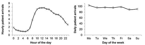 ) shows the average number of patient arrivals at ED3. As expected, there was a significant effect of the hour of the day on the number of arrivals, F(23, 24672) = 1043.13, p < .001, η2 = .49. The effect size (η2) indicates that the hour of the day explained 49% of the variance in the number of hourly arrivals. There was also a significant effect of the day of the week on the number of arrivals, F(6, 1022) = 15.95, p < .001, η2 = .09. However, the effect size was moderate in that the day of the week merely explained 9% of the variance in the number of daily arrivals. In addition, the month of the year explained 7% of the variance in the number of daily arrivals, F(11, 1017) = 7.46, p < .001, η2 = .07. The pattern in patient arrivals was similar for the three other EDs. Specifically, the effect sizes for the effect of the hour of the day on the number of arrivals were 51% (ED1), 53% (ED2), and 52% (ED4).
After having confirmed the importance of calendar variables to the number of patient arrivals (see Fig. 1), we turned to the creation of the forecasting models. To recap, the regression models had indicator variables for the hours of the day, the days of the week, and the months of the year, the ARIMA models had a season consisting of the 168 hours of the week, and the naïve models used the number of arrivals at the same time last week as their prediction. The coefficients of the resulting regression models (see Appendix 1) showed larger variation in patient arrivals across the hours of the day than across the days of the week and the months of the year. In terms of the hour of the day, patient arrivals peaked at 11 (ED1), 12 (ED2), 13 (ED3), and 11 (ED4). For all four EDs, Monday was the busiest day; Saturday and Sunday were the quietest. The month with the highest number of patient arrivals was July-August (ED1), September (ED2), May (ED3), and September (ED4), while the month with the lowest number of arrivals was either January or February. With respect to the resulting ARIMA models it can be noted that they all had a non-seasonal component (all ps and qs were non-zero, see Table 3) as well as a seasonal component (all Ps and Qs were non-zero, see Table 3). That is, the forecasts depended on the immediately preceding values in the time series as well as on the values for the same time the preceding weeks. In addition, none of the ARIMA models had a global trend (all ds and Ds were zero). That is, throughout each data series the number of patient arrivals varied about an unchanging mean level.
 |
Fig. (1) Number of patient arrivals at ED3 by hour of the day and day of the week. Note: Data for 1029 days. Error bars show the 95% confidence interval. |
Table 3 summarizes the accuracy of the models. The models forecasted the number of patient arrivals during every hour of January 2015 with a mean error of 1.62-1.82 (regression), 1.59-1.82 (ARIMA), and 2.19-2.36 (naïve) patients, corresponding to mean percentage errors of 47% or more. Four issues should be noted. First, the accuracy was similar across EDs, thereby increasing the robustness of the results. Second, the models did not describe the data used in building the models with better accuracy than the accuracy with which they forecasted arrivals occurring after the data used in building the models. This similarity of the in-sample accuracy and the out-of-sample accuracy indicated that the models did not overfit the data. Third, the regression and ARIMA models were an improvement over the naïve model but only a moderate improvement. The forecast errors were 73-77% (regression) and 72-75% (ARIMA) of the errors obtained with the naïve model. Fourth, the accuracy of the regression models and the ARIMA models was near identical.

A possible reason for the modest accuracy of the models was the short forecasting interval. In the number of hourly arrivals, the pattern caused by calendar variables might not contain enough patients to overshadow the noise caused by random variation. To investigate this possibility we created models with forecasting intervals of 2, 4, 8, and 24 hours. Table 4 shows the accuracy of these models for ED2; the models for the other EDs had similar accuracies. There was a consistent decrease in mean percentage error as the forecasting interval increased. With a forecasting interval of 24 hours (i.e., forecasting the number of daily arrivals), the mean percentage error of the forecasts had decreased to 9.9% (regression) and 11% (ARIMA). A forecasting interval of 8 hours, corresponding to a work shift, still yielded forecasts with a mean percentage error of 26% (regression) and 21% (ARIMA). For all four EDs the ARIMA models were more accurate than the regression models at forecasting intervals of 2, 4, and 8 hours, whereas the results at a forecasting interval of 24 hours were mixed. The improvement over the naïve model remained moderate at all forecasting intervals.
3.2. ED Occupancy
Fig. (2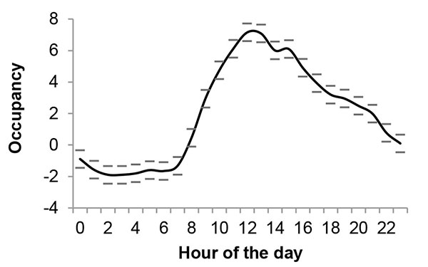 ) shows the occupancy of ED1. There was a significant effect of the hour of the day on the occupancy of ED1, F(23, 17280) = 126.04, p < .0001, η2 = .14. The occupancy increased steeply from 7 in the morning until noon and then decreased gradually the rest of the day. The pattern was roughly similar for the other EDs but the effect sizes varied. That is, the hour of the day explained 14% (ED1), 33% (ED2), 32% (ED3), and 2.2% (ED4) of the variance in occupancy.
 |
Fig. (2) Occupancy in terms of the accumulated increase since midnight in the number of patients in ED1. Note: Data for 721 days. Error bars show the 95% confidence interval. |
We created forecasting models for the occupancy of the EDs. The models forecasted the occupancy during every hour of January 2015 with a mean error of 5.40-17.71 (regression), 2.57-5.43 (ARIMA), and 7.29-23.63 (naïve) patients, see Table 5. For each model, the errors were similar for ED1, ED2, and ED3 but markedly larger for ED4. The larger errors for ED4 were unsurprising given the negligible size of the effect of the hour of the day on the occupancy of ED4. However, even for ED1 to ED3 the mean percentage error of the forecasts was at least 69%. We note that the forecast errors were 23-37% (ARIMA) and 72-75% (regression) of the errors obtained with the naïve model. Thus, the ARIMA models were substantially more accurate than the naïve and regression models. We also note that the models did not overfit the data, as indicated by the similarity of the in-sample and out-of-sample accuracies.
To begin to understand the influence of throughput and output, as opposed to input, factors on the occupancy of the EDs, we looked at the patients’ length of stay in the ED. By comparing whether length of stay was affected more by the hour of the day at which the patient arrived in the ED or the hour of the day at which the patient left the ED, we got an indication of the relative influence of input and output factors on ED occupancy. Fig. (3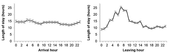 ) shows these data for ED4. Arrival hour explained a negligible 0.5% of the variance in length of stay, whereas leaving hour explained 6.0%. Across the four EDs, arrival hour explained 0.5-0.8% and leaving hour 4.1-15% of the variance in length of stay. Leaving hour explained an average of 12 times more of the variance than arrival hour, thereby suggesting that more accurate forecasting models of ED occupancy can be created by introducing factors beyond calendar variables.
 |
Fig. (3) Length of stay by the hour of the day at which the patient arrived in ED4 and left ED4. Note: Data for 1029 days. Error bars show the 95% confidence interval. |
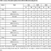
In addition to calendar variables, the log data contained information about, among other things, the patients’ progress through the ED workflow. The EDs recorded different sets of such throughput information but the workflows of the EDs shared five main activities: triage, waiting to be seen by nurse, waiting to be seen by physician, examination (by junior physician), and review (by senior physician). Information about the patients’ progress through these activities was included on the whiteboard because at-a-glance access to this information was deemed important to the ED clinicians’ overview of the state of the ED. Yet, the log data showed that even these five main treatment activities were recorded for only a subset of the ED visits, see Table 6. For example, triage was only recorded as the current treatment activity for 0.02-28% of the ED visits. Importantly, this does not indicate that a minority of the patients were triaged but that triage was only documented as the current treatment activity for a minority of the patients. The lack of consistency with which these throughput factors were recorded prevented their use in forecasting models.

4. DISCUSSION
In the following, we discuss the accuracy of the forecasts, the data necessary to make more accurate forecasts, and the limitations of this study.
4.1. Accuracy of the Forecasts
The regression and ARIMA models forecasted hourly arrivals with an absolute error (MAE) of 1.59-1.82 patients, corresponding to a percentage error (MAPE) of 47-58%. These results accord with the few previous studies that have looked at hourly forecasts. Using a multivariate time-series model, Jones et al. [22Jones SS, Evans RS, Allen TL, et al. A multivariate time series approach to modeling and forecasting demand in the emergency department. J Biomed Inform 2009; 42(1): 123-39.
[http://dx.doi.org/10.1016/j.jbi.2008.05.003] [PMID: 18571990] ] forecasted hourly patient arrivals with an MAE of approximately two patients for three EDs seeing slightly more patients than the EDs in this study. Using a tailor-made model, Boyle et al. [23Boyle J, Jessup M, Crilly J, et al. Predicting emergency department admissions. Emerg Med J 2012; 29(5): 358-65.
[http://dx.doi.org/10.1136/emj.2010.103531] [PMID: 21705374] ] forecasted hourly arrivals with an MAPE of 50%. Given the measures of the accuracy of the forecasts, can the models be considered accurate? This question warrants four notes.
First, Jones et al. [22, pJones SS, Evans RS, Allen TL, et al. A multivariate time series approach to modeling and forecasting demand in the emergency department. J Biomed Inform 2009; 42(1): 123-39.
[http://dx.doi.org/10.1016/j.jbi.2008.05.003] [PMID: 18571990] . 135] were “pleased with the high degree of accuracy” of their model. It also speaks to the advantage of our models that they do not overfit the data. In addition, models that extend calendar variables with weather variables, such as temperature readings and rain-/snowfall data, do not achieve better accuracy [24Wargon M, Guidet B, Hoang TD, Hejblum G. A systematic review of models for forecasting the number of emergency department visits. Emerg Med J 2009; 26(6): 395-9.
[http://dx.doi.org/10.1136/emj.2008.062380] [PMID: 19465606] ]. Adding variables about the demand for inpatient resources has also been found not to improve the accuracy of models of ED visits [22Jones SS, Evans RS, Allen TL, et al. A multivariate time series approach to modeling and forecasting demand in the emergency department. J Biomed Inform 2009; 42(1): 123-39.
[http://dx.doi.org/10.1016/j.jbi.2008.05.003] [PMID: 18571990] ].
Second, the percentage error of the forecasts increased as the forecast interval decreased. The forecasts of the ARIMA models for ED2 had a percentage error of 11% for daily arrivals, 21% for 8-hourly arrivals, 34% for 4-hourly arrivals, 41% for 2-hourly arrivals, and 49% for hourly arrivals. This finding is important because it shows that MAPE values for one forecast interval do not generalize to other forecast intervals. Rather, forecasts of hourly arrivals are less accurate than forecasts of daily arrivals. It may be noted that the MAPE of 11% for daily arrivals in ED2 is within the range (4.2-14.4%) reported by Wargon et al. [24Wargon M, Guidet B, Hoang TD, Hejblum G. A systematic review of models for forecasting the number of emergency department visits. Emerg Med J 2009; 26(6): 395-9.
[http://dx.doi.org/10.1136/emj.2008.062380] [PMID: 19465606] ] in a review of models for forecasting the number of daily ED visits, thereby suggesting that a worsening of the MAPE from 11% (daily) to 49% (hourly) may not be unusual. Part of the reason for the worse MAPE for hourly arrivals likely is that the averaging approach of the models means that they underestimate the level of short-term variability and the size of occasional surges [15Wiler JL, Griffey RT, Olsen T. Review of modeling approaches for emergency department patient flow and crowding research. Acad Emerg Med 2011; 18(12): 1371-9.
[http://dx.doi.org/10.1111/j.1553-2712.2011.01135.x] [PMID: 22168201] ].
Third, the extra complexity of the regression and ARIMA models relative to the naïve model resulted in smaller errors. In modeling patient arrivals, the regression and ARIMA models performed similarly for all forecast intervals. This result accords with previous studies of daily arrivals [8Jones SS, Thomas A, Evans RS, Welch SJ, Haug PJ, Snow GL. Forecasting daily patient volumes in the emergency department. Acad Emerg Med 2008; 15(2): 159-70.
[http://dx.doi.org/10.1111/j.1553-2712.2007.00032.x] [PMID: 18275446] ]. In modeling ED occupancy, the ARIMA models were superior to the regression models, but it should be kept in mind that the models of occupancy were less accurate than those of arrivals. Furthermore, the multivariate time-series model used by Jones et al. [22Jones SS, Evans RS, Allen TL, et al. A multivariate time series approach to modeling and forecasting demand in the emergency department. J Biomed Inform 2009; 42(1): 123-39.
[http://dx.doi.org/10.1016/j.jbi.2008.05.003] [PMID: 18571990] ] did not achieve lower errors than our ARIMA models in spite of the increased complexity of their multivariate approach compared to ARIMA models, which are univariate. These results indicate that ARIMA models are, currently, among the most accurate models for forecasting ED visits.
Fourth, evidence about the use of forecasting models during ED work is scarce, probably because the data necessary to make such forecasts in real time are only gradually becoming available. Thus, it is still mainly future work to assess whether the models provide sufficiently accurate forecasts to be useful in practice. Jessup et al. [25Jessup M, Crilly J, Boyle J, et al. Users' experiences of an emergency department patient admission predictive tool: A qualitative evaluation. Health Informatics J 2016; 22(3): 618-32.
[http://dx.doi.org/10.1177/1460458215577993] [PMID: 25916833] ] studied ED clinicians’ experience of a forecasting tool after it had been in use for a year. The forecasts varied from being experienced as “pretty accurate” on some days to “off the mark” on others. Generally, the interviewees were positive about the tool but did not assign its forecasts any special authority. The main driver of the positive view of the tool appeared to be that it facilitated communication by bringing people together as they accessed the tool and talked about its forecasts. That is, the actual forecasts (and their accuracy) may be less important than the communication and collective decision-making that evolved around the tool. The combined role of communication and content in relation to the forecasting tool resembles studies of the role of ED whiteboards [13Hertzum M, Simonsen J. Visual overview, oral detail: The use of an emergency-department whiteboard. Int J Hum Comput Stud 2015; 82: 21-30.
[http://dx.doi.org/10.1016/j.ijhcs.2015.04.004] ].
4.2. Data for Forecasting
Forecasting requires reliable data. Patients’ arrival in the EDs was consistently recorded, and these calendar data permitted forecasts of hourly patient arrivals with modest but useful accuracy. The hourly ED occupancy could not be forecasted with similar accuracy on the basis of calendar variables. While the ARIMA models forecasted hourly ED occupancy substantially better than the regression and naïve models, the mean percentage error of the ARIMA forecasts was 69-73% for ED1 to ED3 and 101% for ED4. Four issues should be noted in relation to the forecasts of ED occupancy.
First, it appears that additional information may generate more accurate forecasts of hourly ED occupancy. ED occupancy is influenced by the number of patient arrivals as well as by the throughput and output of the ED. The influence of throughput and output factors is illustrated by the better ability of leaving hour than arrival hour to explain the variance in length of stay in the EDs. Abraham et al. [26Abraham G, Byrnes GB, Bain CA. Short-term forecasting of emergency inpatient flow. IEEE Trans Inf Technol Biomed 2009; 13(3): 380-8.
[http://dx.doi.org/10.1109/TITB.2009.2014565] [PMID: 19244023] ] report a similar result for total length of stay in the hospital and propose that the better ability of leaving time to explain variance in length of stay is due to fewer discharges over the weekend and other differences in discharge practices. While this proposition focuses on output factors and bypasses throughput factors, Hertzum [2Hertzum M. Patterns in emergency-department arrivals and length of stay: Input for visualizations of crowding. Ergon Open J 2016; 9: 1-14.
[http://dx.doi.org/10.2174/1875934301609010001] ] lists both throughput and output factors as bottlenecks in the ED. The listed throughput factors include linear workflows and manual data entry. It is, however, not obvious how such factors may be included in forecasting models.
Second, throughput and output factors probably vary more across EDs than input factors because throughput and output factors include hospital issues as well as patient issues. For example, the large differences in average ED length of stay (Table 2) indicate differences in the division of labor between the ED and the inpatient departments. The impact of these issues is, for example, apparent in the substantially larger errors in the forecasts of the occupancy of ED4 compared to the other EDs, and it suggests that the selection of variables for forecasting models of ED occupancy may need to be tailored to local conditions. Conversely, the demographic differences in the catchment areas of the EDs (Table 1) did not lead to marked differences across the EDs in the forecast accuracy of patient arrivals.
Third, we extracted information about the patients’ progress through the ED from the log data with the aim of using this throughput information in the modeling of ED occupancy. We expected that, for example, waiting longer to be seen by a nurse would be a predictor of higher ED occupancy. Instead, we found a frequent absence of information about which treatment activity was currently in progress. Out of five main treatment activities at most one was recorded for more than half of the patients. In all EDs at least one of the five activities was recorded for no more than 17% of the patients. The incomplete recordings prevented the use of these, and other, throughput factors in the forecasting models.
Fourth, the frequent absence of information about which treatment activity was currently in progress is the result of a constant tension between treating patients and documenting treatments. This tension is aggravated by the status of the whiteboard as a transitional artifact. Transitional artifacts hold procedural information and, thereby, fill a gap between the work being performed and the formal documentation of it [27Chen Y. Documenting transitional information in EMR. In: Proceedings of the CHI2010 Conference on Human Factors in Computing Systems. New York: ACM Press 2010; pp. 1787-96.]. Procedural information is pertinent to crowding-related forecasting models but the transitional status of the whiteboard means that the clinicians are not formally required to keep the whiteboard current. As a consequence, it is less consistently kept than the patient records with the formal documentation of the patients’ condition. The introduction of a forecasting tool that presupposes the procedural information might motivate the clinicians to record it more consistently. However, the study by Jessup et al. [25Jessup M, Crilly J, Boyle J, et al. Users' experiences of an emergency department patient admission predictive tool: A qualitative evaluation. Health Informatics J 2016; 22(3): 618-32.
[http://dx.doi.org/10.1177/1460458215577993] [PMID: 25916833] ] suggests that the clinicians may, instead, prefer to interpret and use the forecasts in the light of their knowledge of the imperfect quality of the data on which the forecasts are made. Bypassing manual data entry would resolve this issue but requires that the procedural information can be automatically and reliably derived from other recordings.
4.3. Limitations
Three limitations should be remembered in interpreting the results of this study. First, the data are from EDs in one healthcare region of one country. While the four EDs differ somewhat in demographic characteristics and show that the results of the study are not peculiar to one ED, we acknowledge that the results may be influenced by the Danish healthcare system and by living conditions in Denmark in general. More work is needed on forecasting models of hourly patient arrivals and ED occupancy. Second, the models are restricted by the precision of the data. The models are made from operational data, the recording of which is secondary to the treatment of the patients. Any systematic bias in the recording of the data is reproduced in the models and not brought out in the accuracy measurements because they measure the models against further operational data. A possible bias is that delayed recording may systematically happen more often than early recording. Third, the models have not been tested in use. The accuracy of the model forecasts has been assessed analytically with recognized measures but it remains untested whether the models are useful in the ED to help coordinate work and counteract crowding. A test of the practical usefulness of the models entails the development of a real-time visualization of the forecasts. The development, organizational implementation, and test of such a visualization is important future work.
CONCLUSION
To counteract crowding in the ED, the clinicians need information about how the flow of patients through the ED will evolve in the immediate future. While previous research has mainly focused on forecasting daily or monthly patient arrivals, this study provides models for forecasting patient arrivals and ED occupancy hour by hour on the basis of calendar variables. Hourly forecasts support clinicians in their ongoing scheduling and rescheduling of how the available ED resources are to be divided among the patients in need of ED services. In contrast, daily and monthly forecasts target issues such as staff allocation.
For patient arrivals, regression and ARIMA models performed similarly. Hourly patient arrivals were forecasted with a mean percentage error of 47-58% (regression) and 49-58% (ARIMA) across the four EDs. The forecasts of hourly patient arrivals were substantially less accurate than forecasts of daily patient arrivals. For ED occupancy, ARIMA models were superior to regression models but the errors were larger than for patient arrivals and varied more across the EDs. Hourly ED occupancy was forecasted with a mean percentage error of 69-101% (ARIMA). The error was largest for the ED in which the patients stayed the longest, thereby indicating that with increasing length of stay calendar variables became an increasingly insufficient basis for forecasting occupancy. Apart from this difference, the models performed similarly for the four EDs, which were from the same Danish healthcare region but differed in the demographics of their catchment areas and in the division of labor between the ED and the inpatient departments. This shows that the models may be useful in regional coordination as well as in the individual EDs. More work is needed to ascertain whether the accuracy of the hourly forecasts generalizes beyond the studied healthcare region.
ED occupancy depends on factors beyond calendar variables. However, the use of throughput and output factors in forecasting models presupposes that information about the flow of patients through the ED is consistently recorded. Such procedural information is often recorded in transient artifacts, the use of which is recommended but not mandatory. The whiteboard providing the data for this study is a case in point. It remains for future work to investigate whether the introduction of a forecasting tool in the ED will motivate the clinicians to record procedural information more consistently or whether they, instead, will interpret the forecasts as crude estimates based on imperfect data.
CONFLICT OF INTEREST
The author confirms that this article content has no conflict of interest.
ACKNOWLEDGEMENTS
This study is part of the Clinical Communication project, which is a research and development collaboration between Region Zealand, Imatis, Roskilde University, and University of Copenhagen. The study was co-funded by Region Zealand. The author is grateful to Rasmus Rasmussen at Imatis for extracting the anonymized log data from the electronic whiteboard.
APPENDIX
Standardized coefficients (β) for the regression models of patient arrivals with a 1-hour forecasting interval.

REFERENCES
| [1] | American College of Emergency Physicians. Crowding. Ann Emerg Med 2006; 47(6): 585. [http://dx.doi.org/10.1016/j.annemergmed.2006.02.025] [PMID: 16713796] |
| [2] | Hertzum M. Patterns in emergency-department arrivals and length of stay: Input for visualizations of crowding. Ergon Open J 2016; 9: 1-14. [http://dx.doi.org/10.2174/1875934301609010001] |
| [3] | Kam HJ, Sung JO, Park RW. Prediction of daily patient numbers for a regional emergency medical center using time series analysis. Healthc Inform Res 2010; 16(3): 158-65. [http://dx.doi.org/10.4258/hir.2010.16.3.158] [PMID: 21818435] |
| [4] | Nielsen RF, Pérez N, Petersen P, Biering K. Assessing time to treatment and patient inflow in a Danish emergency department: a cohort study using data from electronic emergency screen boards. BMC Res Notes 2014; 7: 690. [http://dx.doi.org/10.1186/1756-0500-7-690] [PMID: 25288356] |
| [5] | Rotstein Z, Wilf-Miron R, Lavi B, Shahar A, Gabbay U, Noy S. The dynamics of patient visits to a public hospital ED: a statistical model. Am J Emerg Med 1997; 15(6): 596-9. [http://dx.doi.org/10.1016/S0735-6757(97)90166-2] [PMID: 9337370] |
| [6] | Tandberg D, Qualls C. Time series forecasts of emergency department patient volume, length of stay, and acuity. Ann Emerg Med 1994; 23(2): 299-306. [http://dx.doi.org/10.1016/S0196-0644(94)70044-3] [PMID: 8304612] |
| [7] | Batal H, Tench J, McMillan S, Adams J, Mehler PS. Predicting patient visits to an urgent care clinic using calendar variables. Acad Emerg Med 2001; 8(1): 48-53. [http://dx.doi.org/10.1111/j.1553-2712.2001.tb00550.x] [PMID: 11136148] |
| [8] | Jones SS, Thomas A, Evans RS, Welch SJ, Haug PJ, Snow GL. Forecasting daily patient volumes in the emergency department. Acad Emerg Med 2008; 15(2): 159-70. [http://dx.doi.org/10.1111/j.1553-2712.2007.00032.x] [PMID: 18275446] |
| [9] | Marcilio I, Hajat S, Gouveia N. Forecasting daily emergency department visits using calendar variables and ambient temperature readings. Acad Emerg Med 2013; 20(8): 769-77. [http://dx.doi.org/10.1111/acem.12182] [PMID: 24033619] |
| [10] | Sun Y, Heng BH, Seow YT, Seow E. Forecasting daily attendances at an emergency department to aid resource planning. BMC Emerg Med 2009; 9: 1. [http://dx.doi.org/10.1186/1471-227X-9-1] [PMID: 19178716] |
| [11] | Wargon M, Casalino E, Guidet B. From model to forecasting: a multicenter study in emergency departments. Acad Emerg Med 2010; 17(9): 970-8. [http://dx.doi.org/10.1111/j.1553-2712.2010.00847.x] [PMID: 20836778] |
| [12] | Bergs J, Heerinckx P, Verelst S. Knowing what to expect, forecasting monthly emergency department visits: A time-series analysis. Int Emerg Nurs 2014; 22(2): 112-5. [http://dx.doi.org/10.1016/j.ienj.2013.08.001] [PMID: 24055373] |
| [13] | Hertzum M, Simonsen J. Visual overview, oral detail: The use of an emergency-department whiteboard. Int J Hum Comput Stud 2015; 82: 21-30. [http://dx.doi.org/10.1016/j.ijhcs.2015.04.004] |
| [14] | Iserson KV, Moskop JC. Triage in medicine, part I: Concept, history, and types. Ann Emerg Med 2007; 49(3): 275-81. [http://dx.doi.org/10.1016/j.annemergmed.2006.05.019] [PMID: 17141139] |
| [15] | Wiler JL, Griffey RT, Olsen T. Review of modeling approaches for emergency department patient flow and crowding research. Acad Emerg Med 2011; 18(12): 1371-9. [http://dx.doi.org/10.1111/j.1553-2712.2011.01135.x] [PMID: 22168201] |
| [16] | Thompson ML. Selection of variables in multiple regression: Part I. A review and evaluation. Int Stat Rev 1978; 46(1): 1-19. [http://dx.doi.org/10.2307/1402505] |
| [17] | Box GE, Jenkins GM, Reinsel GC. Time series analysis: Forecasting and control. 4th ed. New York: Wiley 2008. [http://dx.doi.org/10.1002/9781118619193] |
| [18] | Makridakis S, Wheelright S, Hyndman RJ. Forecasting: Methods and applications. 3rd ed. New York: Wiley 1998. |
| [19] | Willmott CJ, Matsuura K. Advantages of the mean absolute error (MAE) over the root mean square error (RMSE) in assessing average model performance. Clim Res 2005; 30(1): 79-82. [http://dx.doi.org/10.3354/cr030079] |
| [20] | Bowerman BL, O'Connell RT, Koehler AB. Forecasting, time series and regression: An applied approach. 4th ed. Belmont, CA: Thomson Brooks/Cole 2004. |
| [21] | Hyndman RJ, Koehler AB. Another look at measures of forecast accuracy. Int J Forecast 2006; 22(4): 679-88. [http://dx.doi.org/10.1016/j.ijforecast.2006.03.001] |
| [22] | Jones SS, Evans RS, Allen TL, et al. A multivariate time series approach to modeling and forecasting demand in the emergency department. J Biomed Inform 2009; 42(1): 123-39. [http://dx.doi.org/10.1016/j.jbi.2008.05.003] [PMID: 18571990] |
| [23] | Boyle J, Jessup M, Crilly J, et al. Predicting emergency department admissions. Emerg Med J 2012; 29(5): 358-65. [http://dx.doi.org/10.1136/emj.2010.103531] [PMID: 21705374] |
| [24] | Wargon M, Guidet B, Hoang TD, Hejblum G. A systematic review of models for forecasting the number of emergency department visits. Emerg Med J 2009; 26(6): 395-9. [http://dx.doi.org/10.1136/emj.2008.062380] [PMID: 19465606] |
| [25] | Jessup M, Crilly J, Boyle J, et al. Users' experiences of an emergency department patient admission predictive tool: A qualitative evaluation. Health Informatics J 2016; 22(3): 618-32. [http://dx.doi.org/10.1177/1460458215577993] [PMID: 25916833] |
| [26] | Abraham G, Byrnes GB, Bain CA. Short-term forecasting of emergency inpatient flow. IEEE Trans Inf Technol Biomed 2009; 13(3): 380-8. [http://dx.doi.org/10.1109/TITB.2009.2014565] [PMID: 19244023] |
| [27] | Chen Y. Documenting transitional information in EMR. In: Proceedings of the CHI2010 Conference on Human Factors in Computing Systems. New York: ACM Press 2010; pp. 1787-96. |