- Home
- About Journals
-
Information for Authors/ReviewersEditorial Policies
Publication Fee
Publication Cycle - Process Flowchart
Online Manuscript Submission and Tracking System
Publishing Ethics and Rectitude
Authorship
Author Benefits
Reviewer Guidelines
Guest Editor Guidelines
Peer Review Workflow
Quick Track Option
Copyediting Services
Bentham Open Membership
Bentham Open Advisory Board
Archiving Policies
Fabricating and Stating False Information
Post Publication Discussions and Corrections
Editorial Management
Advertise With Us
Funding Agencies
Rate List
Kudos
General FAQs
Special Fee Waivers and Discounts
- Contact
- Help
- About Us
- Search


The Open Petroleum Engineering Journal
(Discontinued)
ISSN: 1874-8341 ― Volume 12, 2019
Practical Considerations for Well Performance Analysis and Forecasting in Shale Plays
D. Ilk1, *, T. A. Blasingame2, O. Houzé3
Abstract
Analysis and forecasting of well performance data in unconventional reservoirs is and will likely remain problematic as there is considerable uncertainty related to our current lack of understanding of the fluid flow phenomenon in low/ultra-low permeability reservoir systems.There are many unknowns which are the primary sources of the uncertainty on production performance.To name a few, these can be stated as the link between flow in nano scale and macro scale, effect of natural fractures and stress fields/geomechanics, pressure/stress dependent dynamic reservoir properties (e.g., permeability), Pressure-volume-temperature (PVT) properties at nano scale, extent of drainage area, etc. Recently, a great amount of research has been performed to understand and relate these issues to well performance analysis and forecasting, but still no conclusive answer has been provided.The objective of this paper is to briefly discuss the specifics of flow in low permeability systems and models to represent well performance then present a methodology to analyze and forecast production data.
Article Information

Identifiers and Pagination:
Year: 2016Volume: 9
Issue: Suppl-1, M7
First Page: 107
Last Page: 136
Publisher Id: TOPEJ-9-107
DOI: 10.2174/18748341016090100107
Article History:
Received Date: 25/3/2015Revision Received Date: 29/6/2015
Acceptance Date: 12/8/2015
Electronic publication date: 30/06/2016
Collection year: 2016
open-access license: This is an open access article licensed under the terms of the Creative Commons Attribution-Non-Commercial 4.0 International Public License (CC BY-NC 4.0) (https://creativecommons.org/licenses/by-nc/4.0/legalcode), which permits unrestricted, non-commercial use, distribution and reproduction in any medium, provided the work is properly cited.
* Address correspondence to this author at the DeGolyer and MacNaughton, 5001 Spring Valley Rd. Suite 800 East, USA; E-mail: dilk@demac.com
| Open Peer Review Details | |||
|---|---|---|---|
| Manuscript submitted on 25-3-2015 |
Original Manuscript | Practical Considerations for Well Performance Analysis and Forecasting in Shale Plays | |
1. THE SPECIFICS OF THE DIFFUSION IN SHALE PLAYS
The most obvious difference between conventional and unconventional plays is the order of magnitude of the permeability (i.e., millidarcy and nanodarcy level permeability). Fig. (1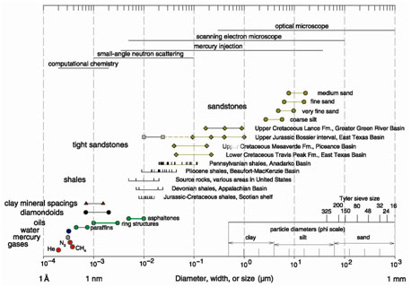 ) presents an illustration of sizes of molecules and pore throats in siliciclastic rocks [1P.H. Nelson, "Pore-throat sizes in sandstones, tight sandstones, and shales", AAPG Bull., vol. 93, pp. 329-430, 2009.
[http://dx.doi.org/10.1306/10240808059] ]. Fig. (2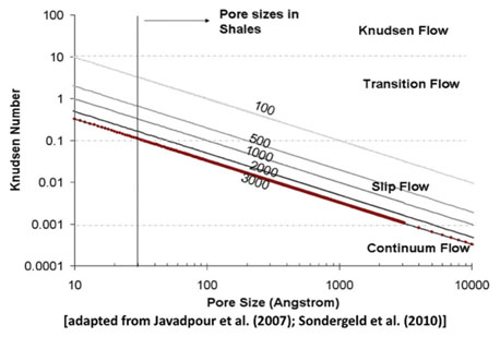 ) presents the Knudsen number (ratio of mean free path of the gas to pore diameter) for methane as a function of pore size for different pore pressure ranging from 100 psi to 3,000 psi. Without even considering the impact on the validity of the diffusion equations, and even considering unreasonably simple flow geometries, the ultra-low permeability alone will have substantial impact as follows:
- The flow is likely to be transient for most of the producing life of the well.
- There are additional challenges to accurately model the system, either analytically or numerically.
- Because we are at the beginning of the production of these types of plays, we totally lack empirical knowledge of their long term production.
Then we have to question the diffusion equations we have been routinely using in the past century. A diffusion equation in a homogeneous context will be the combination of a pressure gradient law (e.g. Darcy), the principle of conservation of mass and a PVT correlation. For the gradient law, the rock constant (e.g. permeability) may be sensitive to pressure and stress. Finally the reservoir may not be homogeneous and may require to be modelled using various networks of natural fractures and matrix blocks.
The diffusion equation resulting from these components is complemented by initial and boundary conditions. In a
conventional play we will reasonably start with uniform pressures and saturations. Inner boundary conditions are mainly about the wells, using pressure gradient law such as Darcy’s law. In a conventional well test the outer boundary conditions may be approximated by an infinite reservoir, but for longer term diffusion one will typically use pressure support (e.g., aquifers) or no-flow boundaries, either physical or coming from the definition of the well drainage area.
Compared to conventional plays, we might still believe in the conservation of mass but all the rest above can and should be challenged:
- The diffusion equations are more complex, and it is accepted that one should consider at least three different scales of diffusion.
- Rock properties are highly dependent on stress.
- With pore size and molecular size approaching the same order of magnitude, PVT correlations derived using "bulk" lab experiments may be challenged.
- Initial producing conditions come after massive hydraulic fracture stimulation treatments. Initial conditions should take into account important pressure and saturation gradients at the initial production time.
- In order to compensate the drop in permeability we increase the magnitude of the contact area between the well and the formation by the means of running multiple fractures along a drain that is generally horizontal. So the well models are much more complex, even assuming we exactly know the fractures geometries, which is seldom the case.
- The last and main challenge today is our lack of knowledge of the flow geometry in the reservoir, and the need (or not) to use discrete fracture networks (DFN).
- To add insult to injury, we typically lack quality data in shale plays.
2. BASIC PRODUCTION BEHAVIOR OF A SHALE WELL
In order to illustrate the basic production behavior of a well in a shale play, we first consider the simplest possible model using typical parameter values. We ignore the complex elements described in the introduction and start with the following assumptions:
 |
Fig. (1) Sizes of molecules and pore throats in siliciclastic rocks [1P.H. Nelson, "Pore-throat sizes in sandstones, tight sandstones, and shales", AAPG Bull., vol. 93, pp. 329-430, 2009. [http://dx.doi.org/10.1306/10240808059] ]. |
 |
Fig. (2) Knudsen number for methane as a function of pore size for various pore pressures at 100°C. This figure illustrates the potentialtypes of gas flow in smaller size pores such as shale based on a Knudsen number.For example, for high pore pressure and Knudsen number less than 0.01, continuum flow (or Darcy flow) is applicable [2C.H. Sondergeld, K.E. Newsham, J.T. Comisky, M.C. Rice, and C.S. Rai, "Petrophysical considerations in evaluating and producing shale gas resources", In: Paper SPE 131768 Presented at the SPE Unconventional Gas Conference, Society of Petroleum Engineers, 23-25 February, Pittsburgh, PA, Pennsylvania, 2010. [http://dx.doi.org/10.2118/131768-MS] ]. |
- Formation Conditions
- — Uniform initial pressure
- — No desorption or other chemical/thermodynamic effects
- — Single-phase flow
- — Homogeneous diffusion using Darcy’s law
- — No microscale heterogeneous behavior
- — No macroscale fracture network
- Multi-Fractured Horizontal Well
- — Fractures have the same length, width, and permeability
- — Fractures are orthogonal to the horizontal well
- — Fractures are placed evenly along the horizontal section
- Well Stimulation
- — The fracturing process is not modelled
- — Water invasion due to stimulation is not modelled
- — Pressure and saturation gradients due to stimulation are not modelled
Although this model is very simplified, this was more or less the state-of-the-art five years ago. For our purposes, we simulate production at a constant pressure for as long as it takes to observe the main flow regimes. Model parameters include a permeability value of 10-4 md, 200 ft effective fracture half-length, 4,000 ft horizontal well length and 40 transverse hydraulic fractures centered in a 5,000 acre (20.9 km2) reservoir with 100 ft thickness, 30 percent initial water saturation, 3 percent porosity and initial reservoir pressure of 5,000 psia. We present the response on a Rate Transient Analysis (RTA) log-log plot, where rate normalized pressure (or pseudopressure) drop is plotted versus material balance time (i.e., instantaneous cumulative production is divided by instantaneous rates).
Although an analytical model should qualitatively reproduce the same log-log response, we utilize the numerical model in order to visualize the pressure fields, which is critical to assess the Stimulated Reservoir Volume (SRV). For each time we present the log-log RTA plot (response curves are given as rate normalized pressure drop and its' Bourdet derivative), the global pressure profile in the reservoir and a close-up look around the well. On each plot green and red dots refer to the time in which a specific flow regime takes place.
In theory, a test long enough to observe the final pseudo steady-state reservoir behavior (PSS) would take several thousand years and the corresponding flowrates during very late times would approach infinitesimal values. However this example is useful for reservoir engineers with a Pressure Transient Analysis (PTA) background to orient themselves regarding the various flow regimes.
2.1. The 'Early' Time Linear Flow Regime
The first series of plots shows the response (i.e., rate normalized pressure drop and its' Bourdet derivative) after one month. When the production is started the flow is linear and orthogonal to the individual fractures. Because of the very low permeability, interference between the fractures is not seen at this stage. The well behaves as a single equivalent fracture with the total length of the individual fractures.
This linear flow is characterized by a half slope on the log-log plot for both normalized pressure and Bourdet derivative, with a factor of 2 between the two curves. Fig. (3 ) illustrates this behavior and the pressure distribution around the horizontal well and fractures. It would also be characterized by a linear trend on a square root of time plot, similar to what is used in PTA for a single hydraulic fracture.
If we were to construct a straight line on an Arps plot we would obtain a "b" factor of 2.
 |
Fig. (3) Simulation response after 1 month. Linear flow regime (characterized by half slope) is observed. Pressure distribution at 1 month is shown. |
2.2. Transition from Linear Flow Regime to SRV Flow Regime
The fractures then begin to interfere. In this example, the next series of figures below show the response after three months. In Fig. (4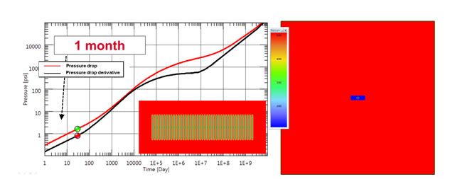 ) both normalized pressure and Bourdet derivative begin to deviate upwards from the half-slope of the linear flow regime. There is a loss of productivity for the well.
Fig. (5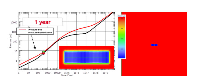 ) shows the end of the transition from linear flow as both normalized pressures and derivatives tend to merge onto a unit slope. In other words effects of the stimulated volume depletion begin to be established. During this transition period, the "b" factor continuously declines from the initial value of 2 (linear flow) and approaches to zero.
 |
Fig. (4) Simulation response after 3 months. Deviations from half slope are observed due to fracture interference. Pressure distribution at 3 months is shown. |
2.3. SRV Flow Regime
For a long period of time both normalized pressure and Bourdet derivative remain on this unit slope, as shown below in Fig. (6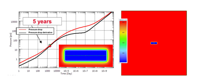 ) after five years. This regime is called "SRV flow", and it is similar in behavior to the traditional pseudosteady-state (PSS) in conventional plays.
 |
Fig. (5) Simulation response after one year. Effects of depletion of the stimulated volume begin to be established. Pressure distribution is shown at 1 year. |
The physical explanation is straightforward. During the early phase each fracture produced as if it was alone in the reservoir, and the diffusion is orthogonal to the fracture. Once the interference occurs we are taking the formation "by surprise". There is no diffusion expansion except at the outer face of the two extreme fractures and at the tips of all fractures. This suddenly decreases the contact area between the well and the reservoir, and the only thing left is to deplete the volume already investigated, i.e. the SRV. The SRV flow is a transient behavior that looks like PSS, and some authors call this regime "pseudo-pseudosteady-state" [3B. Song, and C.A. Ehlig-Economides, "Rate-Normalized Pressure Analysis for Determination of Shale Gas Well Performance", In: Paper SPE 144031 presented at the 2011 SPE North American Unconventional Gas Conference and Exhibition, 14-16 June, 2011, The Woodlands, TX, USA, 2011.
[http://dx.doi.org/10.2118/144031-MS] ].
During the SRV flow the "b" factor approaches zero.
 |
Fig. (6) Simulation response after five years. Flow regime corresponds to the depletion of the so-called stimulated reservoir volume. Pressure distribution at 5 years is shown. |
2.4. Beyond SRV
Depending on the reservoir parameters and the well-fractures system, one may see (or not) the response deviates from SRV flow once the contribution of the outer part of the SRV becomes non-negligible. Figs. (7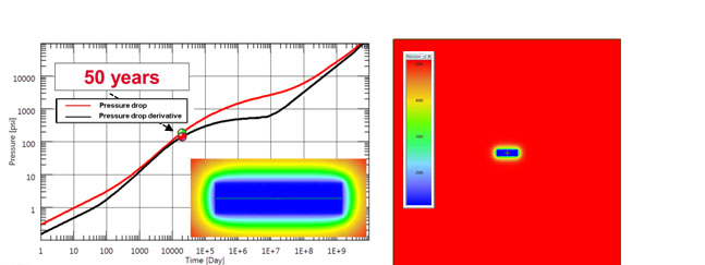 & 9
& 9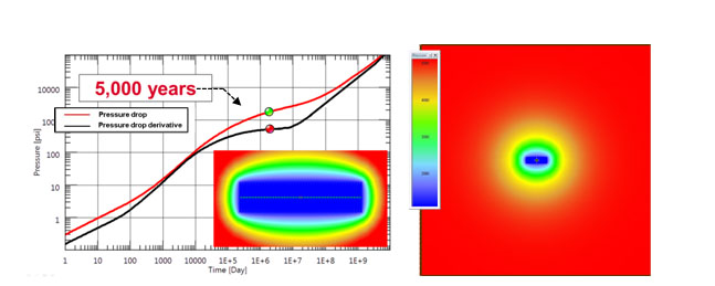 ) demonstrate the deviation from SRV flow regime towards Infinite Acting Radial Flow Regime at 50, 500, and 5,000 years. If we live long enough, we could even see the system reaching the more traditional Infinite Acting Radial Flow (IARF). However this is very unlikely to happen as, by this time, the production would become infinitesimal and the well would be long abandoned. In addition, one would expect that other fractured horizontal wells would have been drilled, completed and produced in the meantime.
 |
Fig. (7) Simulation response after fifty years. Deviations from SRV flow regime has started. Pressure distribution at 50 years is shown. |
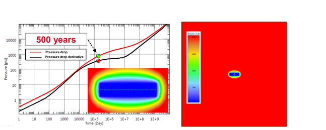 |
Fig. (8) Simulation response after five hundred years. Onset of infinite acting radial flow regime. Pressure distribution at 500 years is shown. |
 |
Fig. (9) Simulation response after five thousand years. Infinite acting radial flow regime is established. Pressure distribution at 5,000 years is shown. |
However, for the sake of the theoretical exercise you will find below in the three next series of plots the response of our example after 50 years, 500 years and 5,000 years, where in our case IARF is reached. We may even want to wait 50,000 years to observe the true PSS as it is shown in Fig. (10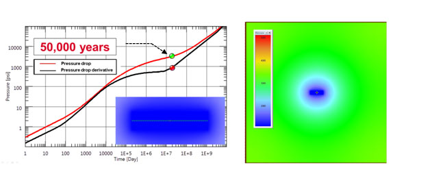 ) below.
 |
Fig. (10) Simulation response after fifty thousand years. Onset of pseudo-steady state flow regime. Pressure distribution at 50,000 years is shown. |
Naturally, this is a theoretical exercise and there are four reasons not to get too much out of it: (1) 50,000 years is indeed a long well test; (2) the whole idea of shale production today is to multiply the number of wells; (3) over long durations simplistic models just fail; (4) even for shorter durations we will see that a number of observations challenge this model.
If we believe this model and return to more realistic production times and abandonment rates, the conclusion is that the meaningful part of the production life of such wells we would see the linear flow, some kind of transition towards the SRV flow, the SRV flow and, depending on the case, some late time deviation if it is not compensated by the production of nearby wells.
This model also represents the position of one of the main schools of thinking around these plays. Beyond the model itself, this school considers that the near totality of the production will come from an SRV that is indeed a slightly inflated version of the bulk volume determined by the series of hydraulic fractures.
This simple model is also a first occasion to introduce the difficulty of forecasting the production of these wells, as shown in Fig. (11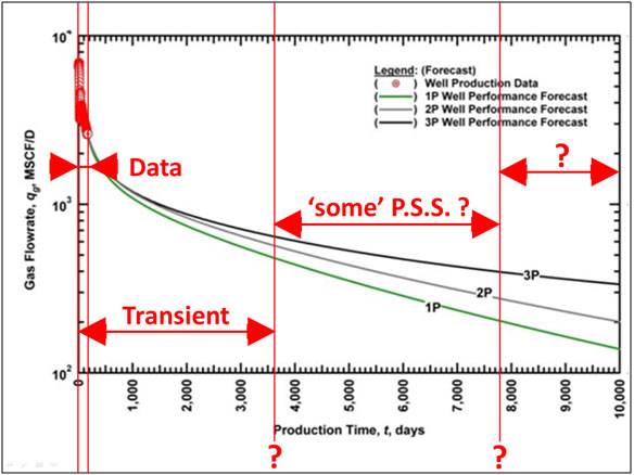 ). We have just been starting to produce these plays and we do not have yet any rule of thumb to extrapolate this data and get an estimate or a probability function for estimated ultimate recovery (EUR).
 |
Fig. (11) Plot of gas flow rate and production time. Possible extrapolations of production data are illustrated. |
3. FIELD EXAMPLE - DEMONSTRATION OF SIMPLE MODELS
To illustrate the basic concepts presented in the previous section we will show the summary of a study done in 2010 with the tools that were then available [4Kappa Engineering, The Analysis of Dynamic Data in Shale Gas Reservoir. Available from: www.kappaeng.com, 2011.]. This horizontal gas well had a length of around 4,000 ft, and 40 hydraulic fractures were expected to be present for an average half-length of around 300 ft. Expected permeability was in the order of 10-4 md, water saturation of 25 percent, pay zone of 100 ft, temperature of 300 °F, initial pressure of 11,000 psia. The well was initially produced from casing, then production was switched to the tubing.
We were initially given 8 months of production data, with both rates and surface pressure. Water flowback was noted during the clean-up (i.e., the first hundred hours of production). A series of analyses were done using the different tools available at the time. All these tools were used to history-match the data and forecasts were generated assuming a constant final flowing pressure. The three forecasts, matching the same data, gave different forecasts and EUR values.
A year later we were given 10 more months of data. We used the results of the three previous interpretations and blindly ran a simulation, but now using the effective 10 months of pressure data. These simulations were compared to the effective 10 months of production to see how these different models behaved in this double-blind process.
3.1. First Eight Months of Production
Rates and surface pressure were provided for the first months of data as shown in Fig. (12a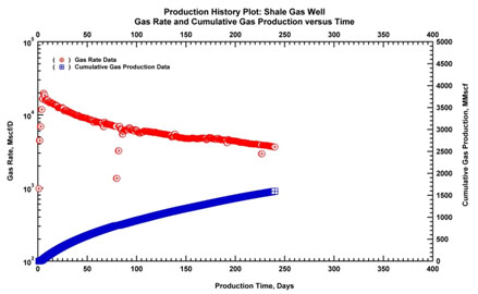 ). Pressure was available at surface and had to be corrected to sandface and plotted in Fig. (12b
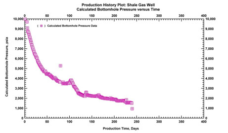 ). Extracting the production we get the log-log plot and the Blasingame plot (Fig. 12c
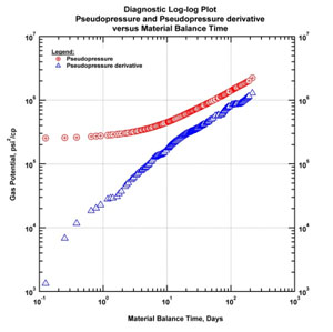 & d
& d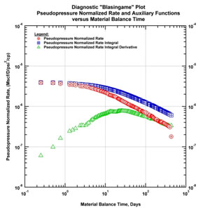 ). Both plots indicate that, after the initial water flowback that dominated for around 100 hours, the main regime during these first months was the linear flow orthogonal to the fractures.
 |
Fig. (12a) Production history plot for 240 days of production. |
 |
Fig. (12b) Calculated bottomhole pressure and time plot for 240 days of production. |
 |
Fig. (12c) Log-log diagnostic plot for 240 days of production. |
 |
Fig. (12d) Diagnostic "Blasingame" plot for 240 days of production. |
3.2. Use of a Single Equivalent Fracture
We begin by focusing on the linear flow regime. A square-root of time plot (Fig. 13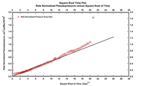 ) would exhibit a linear behavior during this period, allowing an early estimation of k(N.xf)2, where N is the effective number of fractures, k is the matrix permeability and xfthe average fracture half-length.
In order to implement superposition and forecast in the model, we simulated linear flow behavior using the analytical model of a single infinite conductivity fracture in a homogeneous reservoir. The indefinite linear flow from this model was ensured by setting the permeability to an arbitrarily low value. The fracture half-length was then adjusted to match the observed linear flow in the data. A nonlinear regression was then performed. The resulting log-log match and history match are shown in Fig. (14a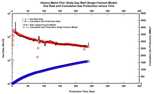 & b
& b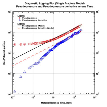 ).
).
 |
Fig. (13) Square root time plot. Straight line is drawn on portions of data which exhibit linear flow behavior. |
 |
Fig. (14a) History match plot using a single fracture model. |
 |
Fig. (14b) History match plot using a single fracture model (log-log diagnostic plot). |
3.3. Analytical Multiple Fractures Horizontal Well (MFHW)
We then used the analytical version of the simple multiple fractures horizontal well described in the previous section. This model accounts for the multi-fracture geometry of the system, and simulates the interferences between them.
The permeability, number of fractures and fracture half-length were set to realistic values. The log-log and history matches are shown in Fig. (15a & b
& b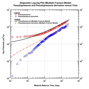 ) after nonlinear regression. The model shows that the interferences between the fractures start after 8 months for this case.
 |
Fig. (15a) History match plot using horizontal well with multiple fractures model (analytical solution). |
 |
Fig. (15b) History match plot using horizontal well with multiple fractures model (log-log diagnostic plot). |
3.4. Numerical MFHW
The same process was applied using the numerical version of the model. Fig. (16a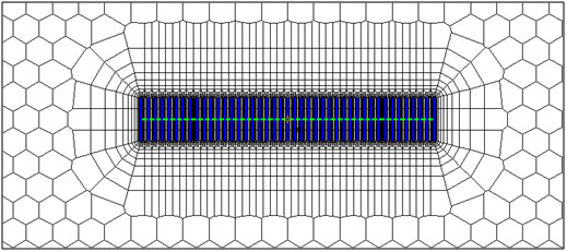 ) below shows the main grid, Fig. (16b
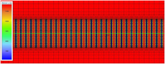 ) shows the pressure distribution around the fractures at one month, from this figure it can be suggested that linear flow regime is observed as flow is orthogonal to each individual fracture. (Fig. 16c
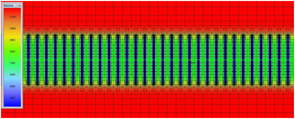 ) shows the pressure distribution around the fractures at eight months. It is observed that flow regime is being deviated from linear flow as fractures seem to be just starting to interfere with each other, the model responses are also shown in Fig. (17a
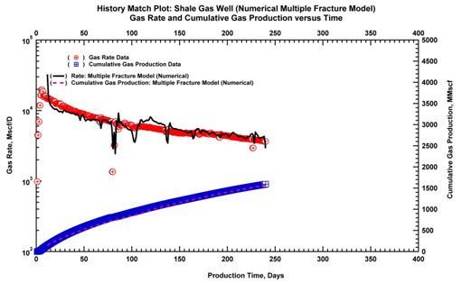 & b
& b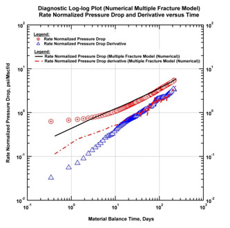 ).
).
 |
Fig. (16a) Unstructured grid blocks for numerical modeling for a multi-frac horizontal well (MFHW). |
 |
Fig. (16b) Pressure distribution at 1 month. Linear flow regime is observed. |
 |
Fig. (16c) Pressure distribution at 8 months. Fractures seem to be just starting to interfere with each other. |
The data was history matched and the resulting log-log and history plots are shown in Fig. (17a & b) below. The apparent noise in the numerical model on the log-log plot comes from the material balance time function. As for the other models a production forecast was then calculated.
 |
Fig. (17a) History match plot using horizontal well with multiple fractures model (numerical solution). |
 |
Fig. (17b) History match plot using horizontal well with "numerical" multiple fractures model (log-log diagnostic plot). |
3.5. Comparing Production Forecasts
The three models described above all match the production data reasonably well given that these models were allowed to converge with different parameters. However, because the underlying assumptions are substantially different they are bound to provide very different long-term production forecasts and EUR values. In Fig. (18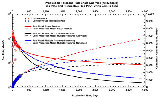 ) the linear flow model, the analytical model and the numerical model are compared with a 10-year forecast using a constant pressure taking the last flowing value.
Fig. (19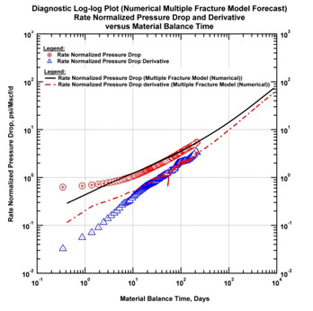 ) below shows the 10-year forecast of the numerical model, as well as the pressure profile after 10 years of production Fig. (20
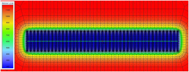 ) presents the pressure distribution at 10 years.
 |
Fig. (18) 10-year forecast of production data (all models). |
 |
Fig. (19) 10-Year production forecast on diagnostic plot (effects of long term SRV flow regime). |
 |
Fig. (20) Pressure profile after 10 years of production. |
3.6. Getting Ten More Months of Production Data
One year later we received 10 more months of data and we checked how our initial forecast matched the observed behavior. Fig. (21a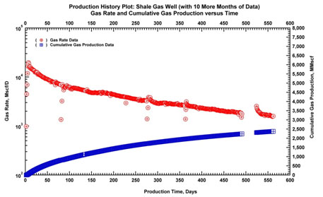 ) illustrates the gas rate and cumulative production with additional data and Fig. (21b
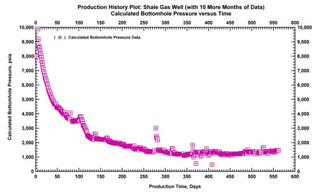 ) illustrates the calculated bottomhole pressure and time with additional data. The data was extracted again on log-log and Blasingame plots Fig. (21c
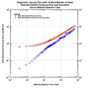 & d
& d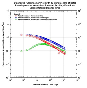 ) and the three models, with the same parameters. The main difference with the initial forecast was that the real producing pressure was used instead of the constant pressure of the previous exercise.
 |
Fig. (21a) Production history plot with additional data (10 more months). |
 |
Fig. (21b) Calculated bottomhole pressure and time plot with additional data (10 more months). |
 |
Fig. (21c) Log-log diagnostic plot with additional data (10 more months). |
 |
Fig. (21d) Diagnostic "Blasingame" plot with additional data (10 more months). |
Fig. (22a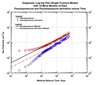 & c
& c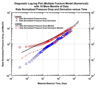 ) show how the three models match the observed response and Fig. (23
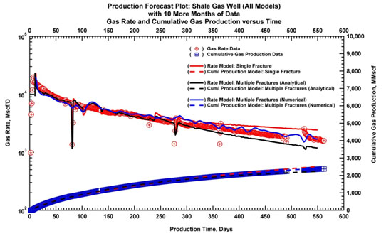 ) presents the history match:
- As expected the single fracture model maintains its initial trend while the observed data deviate due to the interferences between the fractures. The model, which corresponds to a "b" factor of 2, is naturally overly-optimistic.
- As expected again the analytical model (without pseudotime correction) deviates towards SRV flow without taking into account the improvement of the permeability. This model is therefore overly-pessimistic.
- Though the numerical model does not match exactly the data trends, we believe that this model is probably the most consistent approach, and tends to provide the most plausible results.
 |
Fig. (22a) Diagnostic "log-log" plot model match with additional data (Single Fracture Model). |
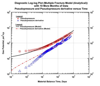 |
Fig. (22b) Diagnostic "log-log" plot model match with additional data (Multiple Fracture Model (Analytical Solution)). |
 |
Fig. (22c) Diagnostic "log-log" plot model match with additional data (Multiple Fracture Model (Numerical Solution)). |
 |
Fig. (23) Comparison of model matches with additional data. |
3.7. Discussion
The example of this section was published in 2011 [4Kappa Engineering, The Analysis of Dynamic Data in Shale Gas Reservoir. Available from: www.kappaeng.com, 2011., 5 Available from: www.kappaeng.com], and we acknowledge that there is no way to prove that this (or any) numerical model is a universal, long-term solution to all our problems. However, we can see from these examples that a relatively simple numerical model carrying the basic assumptions of diffusion and PVT can match pretty well, in some cases, the early years of responses of these wells.
Extrapolating this relatively satisfactory result to long term multiwell production would certainly be an excessive leap of faith. There are actually a lot of mitigating factors:
- Poor data - pressures are only recorded at the surface.
- Operational issues.
- Other elements, such as well interference, well damage, the contribution of natural fractures, a geometric reality much more complex than these simplified models - these conditions clearly highlight the limitations of these simplistic models.
As a result it became clear that these simplified proxies, whether analytical or numerical, may not constitute a satisfactory answer to our long term needs.
4.. DECLINE CURVE ANALYSIS (DCA) OF SHALE PLAYS
The use of DCA in unconventional plays is problematic. A prerequisite to any discussion is the understanding that no simplified time-rate model can accurately capture all elements of performance. The analyst should be realistic and practical when attempting to characterize production performance of systems where permeability is on the order of nanodarcys. Although the hydraulic fractures enable economic production performance, today we only have a basic understanding of the flow structure in the hydraulic and natural fracture systems.
From a historical perspective, Arps' exponential and hyperbolic relations have been the standard for evaluating Estimated Ultimate Recovery (EUR). However, in unconventional plays these relations often yield ambiguous results due to invalid assumptions. The main assumptions which form the basis of traditional DCA can be summarized as:
- There is no significant change in operating conditions and field development during the producing life of the well
- The well is producing with a constant bottomhole flowing pressure
- There is a boundary-dominated flow regime and reservoir depletion was established
In ultra-low permeability reservoirs it is common to observe basic violations of these assumptions, hence the misapplications of the Arps' relations to production data with significant overestimation of reserves, specifically when the hyperbolic relation is extrapolated with a b-exponent greater than 1.
In order to prevent this overestimation, the hyperbolic trend may be coupled with a late time exponential decline. However, this approach remains empirical non-unique, yielding widely varying estimates of reserves.
Numerous authors [6D. Ilk, A.D. Perego, J.A. Rushing, and T.A. Blasingame, "Exponential vs. Hyperbolic Decline in Tight Gas Sands - Understanding the Origin and Implications for Reserve Estimates Using Arps' Decline Curves", In: Paper SPE 116731 Presented at the SPE Annual Technical Conference and Exhibition, 21-24 September, 2008, Denver, CO, Colorado, 2008.
[http://dx.doi.org/10.2118/116731-MS] -9A.N. Duong, "Rate-decline analysis for fracture-dominated shale reservoirs", SPE Reservoir Eval. Eng., vol. 14, no. 3, pp. 377-387, 2011.
[http://dx.doi.org/10.2118/137748-PA] ] have proposed various empirical rate decline relations which attempt to model the time-rate behavior observed in unconventional plays, integrating the early time transient and transitional flow regimes. None of them can extend to all unconventional plays. It is important to understand the applicability of each equation. All of these relations may produce good matches across the entire production time, but each relation may significantly diverge in the forecast and hence the estimation of EUR.
An alternative is to apply all relations in tandem to obtain a range of outcomes rather than a single EUR value. This range of outcomes may be associated with the uncertainty related with production forecast and can be evaluated as a function of time. Fig. (24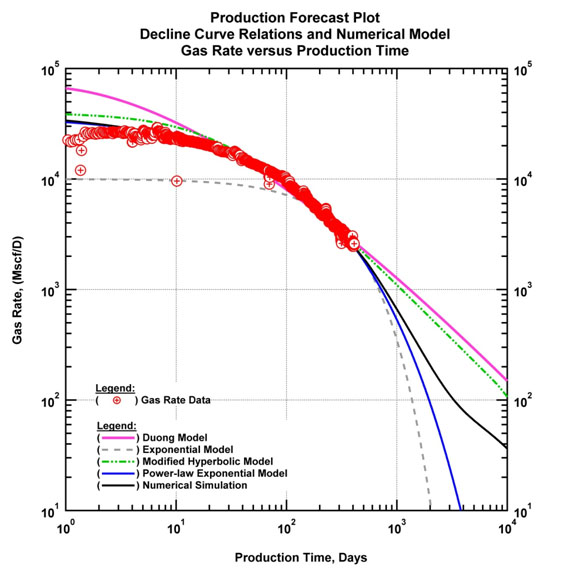 ) presents the application of various decline curve relations to the previously presented shale gas well example. Decline models are plotted along with the numerical model forecast. It can be observed that the forecast from decline curve relations yield a range of EUR values.
5. ANALYTICAL AND NUMERICAL MODELS - TOWARDS INCREASING COMPLEXITY
The simple model described above assumes that all hydraulic fractures share common features: same length, same conductivity, evenly spaced and orthogonal to the horizontal drain. This allows models to be determined using a limited number of parameters: number of fractures, fracture half-length and conductivity. Given the poor level of data we have this is already enough to make the problem under-defined.
However there are cases where one has other information, or sometimes the simple models just do not explain the observed behavior. In such cases you may need to simulate more complex models, with the risk of having insufficient data to nail the problem down.
 |
Fig. (24) (Log-log) Rate and time plot with several DCA models. |
5.1. Complex Geometries (Analytical + Numerical)
The first way to refine the models is to keep the same assumptions related to global homogeneous diffusion equations, but refine the geometry of the hydraulic fractures. We want to substantially increase the range of possible geometries, analytically if we can, numerically if we must.
So the basic model, beyond the even more simplified SRV and bilinear models described earlier assumes a homogeneous infinite reservoir with the simplest case of fractured horizontal well. All fractures have the same length, they are centered on the well drain, orthogonal to this drain and evenly-spaced (Fig. 25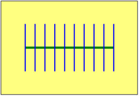 ).
).
 |
Fig. (25) Standard model (analytical and numerical). |
The first step towards a more complex geometry is to allow the fractures to have individual lengths and individual intersection with the well drain. They are still orthogonal to the well and their intersection is at the center of the fracture. This is shown in Fig. (26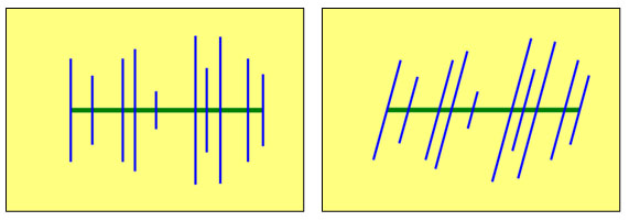 ), right. In complement we can apply a global angle between the well and the set of fractures. This is shown in Fig. (26), left.
 |
Fig. (26) Left: Fractures (individual lengths) + uneven spacing along the well. Right: Fractures + uniform fracture angles. (analytical and numerical). |
Apart from rigorously accounting for nonlinearities, numerical models allow to simulate almost any type of geometry, as long as a suitable grid can be designed. For this reason numerical models can get one step further in terms of flexibility, allowing fractures to have their own angle and an intersection with the horizontal drain that is off-centered as illustrated in Fig. (27 ) below.
 |
Fig. (27) Left: Off-center fractures (individual lengths) + uneven spacing along the well. Right: Off-center fractures + arbitrary fracture angles. (numerical only). |
Since we are working with unstructured grids, the problem consists in rigorously constraining the grid to the direction of the fractures, while ensuring we do not lose the continuous refinements specifically made to capture transients, and without creating too much distortion.
This is a complex yet manageable task, as long as we deal with (1) planar vertical fractures (2) that do not intersect and (3) a cased wellbore. These 3 restrictions being defined, our model is fully flexible: fractures can be non-uniformly distributed along the drain, have different half-lengths and be intercepted by the drain with any (individual) angle or offset.
Fractures can also be partially penetrating (with individual penetrations). In this case, a 3D grid is built (Fig. 28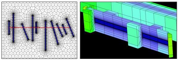 ) around each fracture to ensure that we properly simulate the radial flow from the matrix toward the fracture plane. The drain can intercept the fractures at any depth.
 |
Fig. (28) Left: previous complexity, representation of the grid pattern. Right: 3D refinement for partially penetrating fractures (both numerical only). |
5.2. DFN Models
The next level of complexity is to challenge the assumption that we can model the reservoir response using a more or less complex diffusion equation that would be applied in a homogeneous way. The Discrete Fracture Network (DFN) model considers a network of pre-existing natural fractures that may have been stimulated, or even simply produced after the stimulation jobs. DFN can be combined with the complex hydraulic fracture geometries as mentioned earlier. Given the complexity of the problem and the probable stochastic nature of its definition, the numerical model is the plausible, though it is also possible that numerical DFN can be approximated with analytical solutions (analytical DFN) to get a first estimate of the parameters (density, orientation, etc.) that may be used as a seed to simulate the numerical DFN.
5.3. Example Long-term Production Behavior
To illustrate the effects of complex geometries on production behavior, we simulated three cases. The purpose of this exercise is to have a basic understanding of various geometries on flow behavior and possibly relate these effects to observed behavior in shale plays. We considered three specific cases: (1) horizontal well with multiple fractures in which the fractures are regularly spaced (Fig. 29a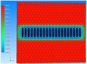 ). This is the most commonly used model and arguably the simplest one. (2) irregularly spaced, off-centered fractures (Fig. 29b
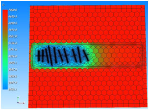 ). The purpose of this configuration is to account for possible in-situ stress effects in fracture propagation and a consideration of inconsistent contribution from each propped fracture along the horizontal well. (3) DFN model (Fig. 29c
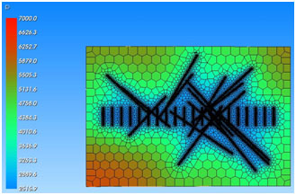 ). This model may represent activated natural fractures or the fracture system around wellbore, and possibly well to well interference if it is used in a multi-well simulation. However, it is not an easy task to set-up the DFN model, and additional constraining data (such as microseismics) is required for this task.
 |
Fig. (29a) Pressure distribution at 30 years.Regularly-spaced fractures. |
 |
Fig. (29b) Pressure distribution at 30 years.Irregularly spaced off-centered fractures (possibly representing contributions from some parts of the wellbore and in-situ stress effects). |
 |
Fig. (29c) Pressure distribution at 30 years.DFN model. |
For each case simulation is run for 30 years and the corresponding pressure distributions are presented below. It is important to note that (1) and (2) models include a stimulated reservoir volume (as defined by the extent of the horizontal well and fracture half-length) and almost no contribution from outside of the stimulated reservoir volume.
Long-term rate profiles obtained from simulation runs are plotted in Fig. (30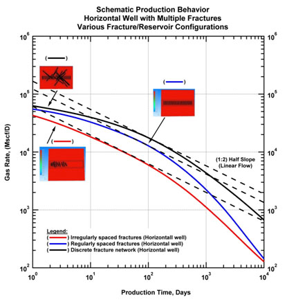 ) below. This schematic illustrates possible production behavior considering the complexities due to well/reservoir/fracture configurations. It is worthwhile to note that linear flow signature (dashed lines) is observed for each case at relatively early times. Rate profiles tend to deviate from linear flow behavior when the effects of SRV depletion are being established. Considering these cases, where same reservoir properties are used for each case, one can assess the effect of completion efficiency by mainly quantifying the vertical separations.
 |
Fig. (30) Long term rate profiles for each simulation case. |
It is worth noting that each case exhibits linear flow (as one could expect). This means that one can easily use a horizontal well model with regularly-spaced fractures to match production data reasonably well (although we recognize that the reality could be different than the idealized model). This brings up the importance of additional data such as production logs, microseismic data, well completion details, etc. for constraining the reservoir model.
6. WORKFLOW FOR THE ANALYSIS AND FORECASTING OF WELLS IN UNCONVENTIONAL RESERVOIRS
In this section we briefly describe a workflow for the analysis and forecasting of multiple wells in unconventional reservoirs. This workflow includes the following steps:
- Production Diagnostics
- - Data quality control
- - Flow regime identification
- - Identification of characteristic behavior
- Model-based Analysis and Forecast of the Representative Well
- Extension of the Model Forecast to Remaining Wells in the Group
The primary objective of this workflow is to efficiently process groups of wells producing in unconventional reservoirs in a fast, yet vigorous way. To that end the steps above are critical, and it is imperative that the first step (production diagnostics) has to be taken into account. We provide an example below in which almost 30 wells are producing in a hypothetical shale play (Fig. 31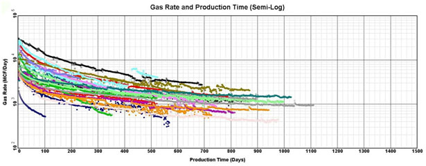 ).
).
 |
Fig. (31) Production data of all wells. |
6.1. Production Diagnostics
The first step of production diagnostics is to go through each well and evaluate the data quality, identify inconsistencies. A visual inspection is sufficient, but for this purpose multiple plots are recommended (e.g., production history plot (time-pressure, time-rate) and log-log flow regime plots). For example, in Figs. (32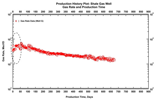 & 33
& 33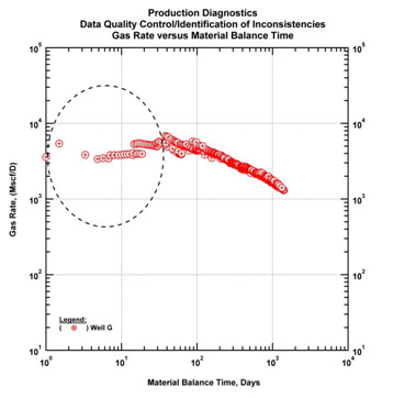 ) below early time well clean-up effects in a producing well are identified by using two plots in tandem. It can be identified from the production history plot that early time clean-up effects (due to flowback) cause an almost flat signature on the log-log flow regime identification plot (rate and material balance time). It is critical to note that these types of inconsistencies or data features should not be confused with actual flow regimes.
 |
Fig. (32) Production history plot (rate and production data).Early time clean-up effects are observed. |
Next and perhaps the most important step of production diagnostics is to identify the flow regimes. For this purpose specific diagnostic plots are used. In particular, these diagnostic plots are log-log plots such as pressure drop normalized rate and time and pressure drop normalized rate and material balance time plots. In the absence of pressure data a constant bottomhole pressure assumption can be made and rate and time/material balance time plots can be used. In this example we process all the wells using the log-log diagnostic plots and identify flow regimes. (Figs. 34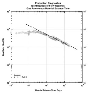 & 35
& 35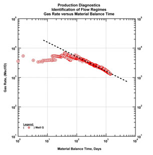 ) are two examples from two wells where linear flow regime is observed to be dominant. Linear flow regime is identified by drawing a half slope on a log-log plot.
 |
Fig. (33) Diagnostic plot (gas rate and gas material balance time). Corresponding early time clean-up effects are identified. |
 |
Fig. (34) Diagnostic plot (gas rate and gas material balance time). Identification of the linear flow regime. |
 |
Fig. (35) Diagnostic plot (gas rate and gas material balance time). Identification of linear flow regime. |
This process is performed for all the wells and common flow regimes and related productivity metrics are identified. With this information groups of similarly performing wells can be created. Fig. (36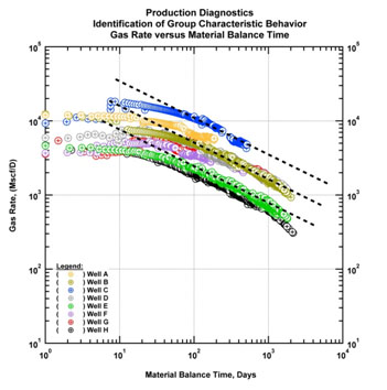 ) below presents a specific group in which the wells are exhibiting similar behavior. In this group the dominant behavior is identified as linear flow and a few wells begin to exhibit indications of the depletion of SRV. This signature is identified by observing deviations from half-slope (linear flow) towards a unit slope on rate and material balance time plot.
 |
Fig. (36) Diagnostic plot (gas rate and gas material balance time). Identification of group characteristic behavior. |
One way to verify characteristic behavior is to use various normalization schemes. Normalization schemes are useful in terms of understanding the important factors affecting production. For example, various completion parameters such as lateral length, number of fracture stages can be used to normalize data (particularly, rates). However, in order to understand if a characteristic behavior is persistent across a group of wells, lump parameters such as cumulative production values of each well at a specific time can be utilized. It is noted that these lump parameters contain the combined effects of reservoir and completion and thus effectively normalize data to reveal a characteristic behavior. In this example normalization by three months cumulative production value (see Fig. (37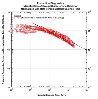 ) below) of each well indicates that the characteristic behavior of this group is linear flow behavior followed by a transitional flow regime, which is likely the depletion of SRV.
 |
Fig. (37) Diagnostic plot (normalized gas rate and gas material balance time). Identification of group characteristic behavior. |
Following the normalization and the identification of characteristic flow regimes, a representative well is selected from the group. This representative well must have sufficient well/reservoir and completion data for rigorous analysis and modeling. Another selection criteria for the representative well includes relatively longer production history with minor inconsistencies compared to the other wells. The production history plot of the representative well is given in Fig. (38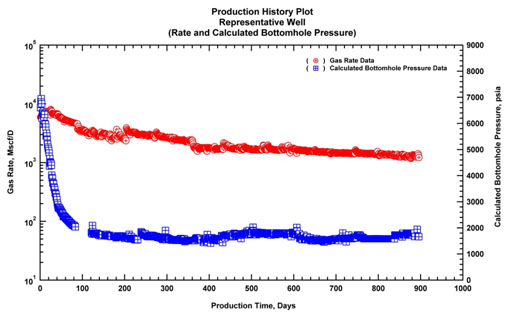 ).
).
 |
Fig. (38) Production history plot of the representative well for modeling. |
6.2. Model-based Analysis:
Based on the selection of the representative well, model-based analysis is performed. Previous sections describe the available models and the applicability of the models to shale plays. In this section we briefly discuss the applicability of three models to our example.
All of these models include a multi-fractured horizontal well (MFHW) configuration. We treat the "drainage area" of the well as the major uncertainty and consider three possibilities: (1) horizontal well with multiple fractures in an infinite acting reservoir, (2) horizontal well with multiple fractures in a closed boundary SRV, which is defined by the extent of the effective fracture half-length, (3) horizontal well with multiple fractures in an SRV, and there is moderate contribution from outside - i.e., analytical trilinear solution (Ozkan 2010) [10E. Ozkan, R. Raghavan, and O.G. Apaydin, "Modeling of fluid transfer from shale matrix to fracture network", In: Society of Petroleum Engineers, SPE Annual Technical Conference and Exhibition, 19–22 September, 2010, Florence, Italy, 2010.
[http://dx.doi.org/10.2118/134830-MS] ]. History matches (i.e., the calculated rate and calculated bottomhole pressure) for these models are presented in Fig. (39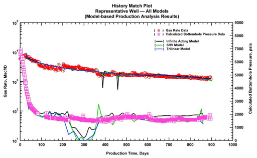 ):
):
 |
Fig. (39) History matches of the representative well. |
As observed in the Fig. (39), each model yields almost identical matches, which confirms the non-uniqueness of the problem. Uncertainty ranges on model parameters (such as permeability, effective fracture half-length, number of fractures, thickness, etc.) can also be considered using a design of experiment methodology for a better understanding of the variability in the production forecasts. However, in this paper we only focus on a brief demonstration of the workflow using simple models and a basic assumption on the uncertainty. The reader is encouraged to consider advanced models with uncertainty ranges for improved well performance analysis and better insights on uncertainty on production forecasts. Back to our example, production forecasts using three models considering the drainage area as the major uncertainty are presented below in Fig. (40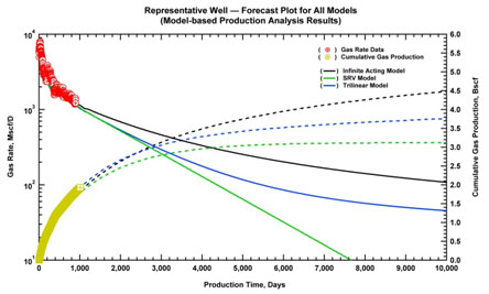 ). It is noted that the estimated ultimate recovery (EUR) ranges between 3.1 Bscf and 4.5 Bscf based on 30 year forecast of production of the representative well.
 |
Fig. (40) Production forecasts of the representative well. |
6.3. Extension to Other Wells
The last step of the workflow is to extend the forecast(s) of the representative well to other wells. Previously we have made the induction that all wells in the group exhibit similar performance behavior and these wells may be represented by a characteristic behavior. Based on this statement we propose that the forecast(s) of the representative well can be extended to other wells by simply applying factors to time and rate data of model forecast - in other words this process can be considered as similar to the type curve matching procedure where data is shifted to obtain the match with the type curve. For our purposes we consider the production data of the well, which the forecast is going to be extended, as static and shift the forecasts on x and y axes to achieve the forecast of the well under consideration. Fig. (41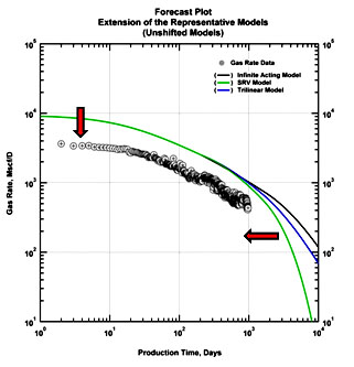 ) illustrates the well, which is not modeled, and the forecasts of the representative well.
 |
Fig. (41) An illustration of extending the representative well forecasts to other wells. |
By applying the x and y factors, forecasts are shifted and matched for the well under consideration. This process is repeated for the remaining wells of the group. The x and y factors are recorded and attempts are made to correlate those with certain productivity metrics (e.g., cumulative production of each well at a specific point in time, say 6 months) and/or completion data (e.g., lateral length). Intuitively one should expect that y-factors are likely correlated with the cumulative production values. So, for the cases where this correlation is not valid, y-factor values for those cases are revisited and matches are refined. This process may serve as a validity check of the process. The extension of the forecasts of the representative well to another well in the group is demonstrated in Fig. (42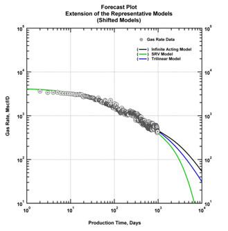 ):
):
 |
Fig. (42) An illustration of extending the representative well forecasts to other wells. (scaled models). |
CONCLUSION
The following conclusions are derived from this study:
- Well performance analysis and forecasting in unconventional reservoir systems is complex - however; a systematic procedure encompassing production diagnostics, simple (time-rate and time-rate-pressure) models, and model-based analysis can be utilized to address various uncertainties and also to establish ranges for production forecasts.
- Model-based production analysis and forecasting is the key to understanding performance characteristics and obtain improved forecasts for ultra-low permeability reservoirs. No other diagnostic can achieve the same objectives of characterizing performance potential. Use of advanced reservoir models is helpful as these models integrate critical information on reservoir description based on subsurface characterization and completion information. However, in the absence of this information, the use of advanced models is problematic, and can lead to an erroneous assessment of reservoir performance capability. In contrast, simple (time-rate and time-rate-pressure) models with certain assumptions for uncertainty ranges on model parameters can be effectively used to establish limits on well performance capability.
- As a summary statement, for ultra-low permeability reservoirs, production diagnostics are the key to understanding well performance behavior prior to analysis and modeling. Production diagnostics must be performed to identify flow regimes as well as establish well groups/clusters based on characteristic well behavior.
DISCLOSURE
This article is an informative up-to-date on the state of the technology published in the book “Dynamic Data Analysis” [5 Available from: www.kappaeng.com].
CONFLICT OF INTEREST
The authors confirm that this article content has no conflict of interest.
ACKNOWLEDGEMENTS
Declared none.
REFERENCES
| [1] | P.H. Nelson, "Pore-throat sizes in sandstones, tight sandstones, and shales", AAPG Bull., vol. 93, pp. 329-430, 2009. [http://dx.doi.org/10.1306/10240808059] |
| [2] | C.H. Sondergeld, K.E. Newsham, J.T. Comisky, M.C. Rice, and C.S. Rai, "Petrophysical considerations in evaluating and producing shale gas resources", In: Paper SPE 131768 Presented at the SPE Unconventional Gas Conference, Society of Petroleum Engineers, 23-25 February, Pittsburgh, PA, Pennsylvania, 2010. [http://dx.doi.org/10.2118/131768-MS] |
| [3] | B. Song, and C.A. Ehlig-Economides, "Rate-Normalized Pressure Analysis for Determination of Shale Gas Well Performance", In: Paper SPE 144031 presented at the 2011 SPE North American Unconventional Gas Conference and Exhibition, 14-16 June, 2011, The Woodlands, TX, USA, 2011. [http://dx.doi.org/10.2118/144031-MS] |
| [4] | Kappa Engineering, The Analysis of Dynamic Data in Shale Gas Reservoir. Available from: www.kappaeng.com, 2011. |
| [5] | Available from: www.kappaeng.com |
| [6] | D. Ilk, A.D. Perego, J.A. Rushing, and T.A. Blasingame, "Exponential vs. Hyperbolic Decline in Tight Gas Sands - Understanding the Origin and Implications for Reserve Estimates Using Arps' Decline Curves", In: Paper SPE 116731 Presented at the SPE Annual Technical Conference and Exhibition, 21-24 September, 2008, Denver, CO, Colorado, 2008. [http://dx.doi.org/10.2118/116731-MS] |
| [7] | P.P. Valkó, "Assigning Value to Stimulation in the Barnett Shale: A Simultaneous Analysis of 7000 Plus Production Histories and Well Completion Records", In: Paper SPE 119369 Presented at the SPE Hydraulic Fracturing Technology Conference, 19-21 January, 2009, College Station, TX, USA, 2009. [http://dx.doi.org/10.2118/119369-MS] |
| [8] | A.J. Clark, L.W. Lake, and T.W. Patzek, "Production Forecasting with Logistic Growth Models", In: Paper SPE 144790 Presented at the SPE Annual Technical Conference and Exhibition, 30 October-02 November, 2011, Denver, CO, Colorado, 2011. [http://dx.doi.org/10.2118/144790-MS] |
| [9] | A.N. Duong, "Rate-decline analysis for fracture-dominated shale reservoirs", SPE Reservoir Eval. Eng., vol. 14, no. 3, pp. 377-387, 2011. [http://dx.doi.org/10.2118/137748-PA] |
| [10] | E. Ozkan, R. Raghavan, and O.G. Apaydin, "Modeling of fluid transfer from shale matrix to fracture network", In: Society of Petroleum Engineers, SPE Annual Technical Conference and Exhibition, 19–22 September, 2010, Florence, Italy, 2010. [http://dx.doi.org/10.2118/134830-MS] |
Endorsements
Browse Contents
Table of Contents
- THE SPECIFICS OF THE DIFFUSION IN SHALE PLAYS
- BASIC PRODUCTION BEHAVIOR OF A SHALE WELL
- The 'Early' Time Linear Flow Regime
- Transition from Linear Flow Regime to SRV Flow Regime
- SRV Flow Regime
- Beyond SRV
- FIELD EXAMPLE - DEMONSTRATION OF SIMPLE MODELS
- First Eight Months of Production
- Use of a Single Equivalent Fracture
- Analytical Multiple Fractures Horizontal Well (MFHW)
- Numerical MFHW
- Comparing Production Forecasts
- Getting Ten More Months of Production Data
- Discussion
- DECLINE CURVE ANALYSIS (DCA) OF SHALE PLAYS
- ANALYTICAL AND NUMERICAL MODELS - TOWARDS INCREASING COMPLEXITY
- Complex Geometries (Analytical + Numerical)
- DFN Models
- Example Long-term Production Behavior
- WORKFLOW FOR THE ANALYSIS AND FORECASTING OF WELLS IN UNCONVENTIONAL RESERVOIRS
- Production Diagnostics
- Model-based Analysis:
- Extension to Other Wells
- CONCLUSION